Thursday, December 21, 2017

Windows Server 2016 Remote Desktop from Ubuntu desktop

Summary

In this post, I'll discuss how to set up a remote desktop session from an Ubuntu client to Windows 2016 Server.

Implementation


Windows-side Configuration


Open up Server Manager, Local Server. 


Click on Remote Desktop.  It will be 'Disabled' on Windows 2016 Standard.  With 2016 Essentials, it's enabled by default.


Choose the 'Allow remote connections to this computer' radio button.  Leave the 'Allow connections only...Network Level Authentication' checkbox selected.  More on that later.  The Administrator will be allowed Remote Desktop access by default.  If you want to add other users, go through the 'Select Users' dialog.

Close this window via the 'OK' button.  Remote Desktop will now show 'Enabled' (may require a screen refresh).  Additionally, Windows will automatically open up the necessary ports through its firewall to enable access to Remote Desktop.  

Ubuntu-side Configuration


rdesktop
rdesktop is a commonly-used RDP client on Ubuntu.  It doesn't appear that development of rdesktop has kept up with the times.  In particular, rdesktop does not support the current authorization protocols within Windows - specifically, Network Level Authentication.  That 'Allow...Network Level Authentication' checkbox mentioned above enables NLA.

Below is an example rdesktop command to initiate a Remote Desktop session:
rdesktop -g 1152x864 -r clipboard:CLIPBOARD -r sound:off -x l -P 1.2.3.4 -u "yourusername" -p yourpassword
If NLA is turned up on the Windows server, you'll get this error:
ERROR: CredSSP: Initialize failed, do you have correct kerberos tgt initialized ?
Failed to connect, CredSSP required by server.
If you're determined to use rdesktop, the simplest fix is to uncheck NLA box on the Windows server.  It will work after that, albeit with less security for the RDP connections.

freerdp
An alternative to rdesktop is FreeRDP.  It does support NLA.  You can either install it directly from the freerdp github site or simply install the version that's in the Ubuntu repositories - xfreerdp
sudo apt-get install freerdp-x11
Below is a sample command line that will set up a Remote Desktop session to Windows 2016, with NLA enabled:
xfreerdp /v:1.2.3.4 /u:yourusername /p:yourpassword +clipboard /size:1152x864
Creating a command launcher on the Ubuntu desktop for remote desktop can be accomplished with the command below:
gnome-desktop-item-edit --create-new ~/Desktop
This will launch a dialog window:

Copy/paste the xfreerdp command into the 'Command:' text box.

Copyright ©1993-2024 Joey E Whelan, All rights reserved.

Tuesday, December 19, 2017

Installation of Genesys 8.5 Configuration DB on Oracle

Summary


This post discusses deployment of the Genesys Config DB on to an existing Oracle 11g instance.

Implementation


  • The Config Server installation includes directory of SQL scripts for various RDMS flavors.  The included Oracle scripts below:
  • ls sql_scripts/oracle
    CfgLocale_ora.sql  drop_tables_ora.sql  init_multi_multilang_ora.sql  init_multi_ora.sql
    
  • Installation of these scripts requires use of the Oracle command line tool, sqlplus.  That tool is located in the /u01/app/oracle/product/11.2.0/xe/bin directory.  Adding this directory to your PATH can be accomplished via execution of the included environment script in the same directory. This can also be added to your .bashrc script to automatically get the Oracle environment set up on login
  • . /u01/app/oracle/product/11.2.0/xe/bin/oracle_env.sh
    
  • The individual SQL scripts can now be executed from the sqlplus command line.  Example below. Assumes the command is being executed from the scripts directory.
  • sqlplus
    
    SQL*Plus: Release 11.2.0.2.0 Production on Tue Dec 19 11:39:15 2017
    
    Copyright (c) 1982, 2011, Oracle.  All rights reserved.
    
    Enter user-name: yourusername
    Enter password: yourpassword
    
    Connected to:
    Oracle Database 11g Express Edition Release 11.2.0.2.0 - 64bit Production
    
    SQL> @drop_tables_ora.sql
    
  • An alternative to executing each of the 3 scripts separately is the one-liner below:
  • (echo @init_multi_ora.sql; echo @CfgLocale_ora.sql) | sqlplus yourusername/yourpassword @drop_tables_ora.sql
    

Copyright ©1993-2024 Joey E Whelan, All rights reserved.

Genesys 8.5 on CentOS/RHEL 6: Oracle DB Client Error

Symptom

Upon attempting to start Genesys Configuration Server, the following error appears:
08:24:00.714 Std 05022 Process './dbclient_oracle_64' started
./dbclient_oracle_64: error while loading shared libraries: libclntsh.so.11.1: cannot open shared object file: No such

Solution

Make the Oracle 11g XE library directory accessible during run time for dynamic linking.
  1. Create a file in /etc/ld.so.conf.d.  In this example, I called it oraclexe.conf
  2. Add the following line to that conf file (path to the Oracle libraries):
  3. /u01/app/oracle/product/11.2.0/xe/lib
    
  4. Execute this command as root to update run-time bindings:
  5. ldconfig -v
    

Snippet of output

/u01/app/oracle/product/11.2.0/xe/lib:
 libdbcfg11.so -> libdbcfg11.so
 libsqora.so.11.1 -> libsqora.so.11.1
 libons.so -> libons.so
 libskgxns.so -> libskgxns.so
 libxdb.so -> libxdb.so
 libqsmashr.so -> libqsmashr.so
 libocrb11.so -> libocrb11.so
 libuini11.so -> libuini11.so
 libntcpaio11.so -> libntcpaio11.so
 libclntsh.so.11.1 -> libclntsh.so.11.1
 libldapjclnt11.so -> libldapjclnt11.so
 libocci.so.11.1 -> libocci.so.11.1
 libnjni11.so -> libnjni11.so
 libodm11.so -> libodm11.so
 libskgxp11.so -> libskgxp11.so
 libnnz11.so -> libnnz11.so
 libheteroxa11.so -> libheteroxa11.so
 libclsra11.so -> libclsra11.so
 libnque11.so -> libnque11.so
 libocijdbc11.so -> libocijdbc11.so
 libhasgen11.so -> libhasgen11.so
 libcorejava.so -> libcorejava.so
 libocrutl11.so -> libocrutl11.so
 libemmas11.so -> libemmas11.so
 libodmd11.so -> libodmd11.so
 libskgxn2.so -> libskgxn2.so
 libcell11.so -> libcell11.so
 libocr11.so -> libocr11.so
 libsqlplus.so -> libsqlplus.so
 libhgotrace11.so -> libhgotrace11.so
 libagtsh.so -> libagtsh.so.1.0

Commentary

A common paradigm in software development is to split out commonly used components into libraries.  In the UNIX/Linux world, those libraries are referred to as shared objects (the 'so' in the names above).  One can determine the library requirements of a given binary with the 'readelf' command.  Example below with the Genesys db client for Oracle:
readelf -d dbclient_oracle_64

Output

Dynamic section at offset 0xc2890 contains 28 entries:
  Tag        Type                         Name/Value
 0x0000000000000001 (NEEDED)             Shared library: [libdl.so.2]
 0x0000000000000001 (NEEDED)             Shared library: [librt.so.1]
 0x0000000000000001 (NEEDED)             Shared library: [libclntsh.so.11.1]
 0x0000000000000001 (NEEDED)             Shared library: [libstdc++.so.6]
 0x0000000000000001 (NEEDED)             Shared library: [libm.so.6]
 0x0000000000000001 (NEEDED)             Shared library: [libgcc_s.so.1]
 0x0000000000000001 (NEEDED)             Shared library: [libpthread.so.0]
 0x0000000000000001 (NEEDED)             Shared library: [libc.so.6]
 0x000000000000000f (RPATH)              Library rpath: [/release/lib/oracle/i686-linux-rhe5/11.2.0/lib64]
 0x000000000000000c (INIT)               0x429558
 0x000000000000000d (FINI)               0x4998f8
 0x000000006ffffef5 (GNU_HASH)           0x400240
 0x0000000000000005 (STRTAB)             0x4140c8
 0x0000000000000006 (SYMTAB)             0x405008
 0x000000000000000a (STRSZ)              73271 (bytes)
 0x000000000000000b (SYMENT)             24 (bytes)
 0x0000000000000015 (DEBUG)              0x0
 0x0000000000000003 (PLTGOT)             0x6c2ee8
 0x0000000000000002 (PLTRELSZ)           3672 (bytes)
 0x0000000000000014 (PLTREL)             RELA
 0x0000000000000017 (JMPREL)             0x428700
 0x0000000000000007 (RELA)               0x427410
 0x0000000000000008 (RELASZ)             4848 (bytes)
 0x0000000000000009 (RELAENT)            24 (bytes)
 0x000000006ffffffe (VERNEED)            0x427310
 0x000000006fffffff (VERNEEDNUM)         6
 0x000000006ffffff0 (VERSYM)             0x425f00
 0x0000000000000000 (NULL)               0x0

Copyright ©1993-2024 Joey E Whelan, All rights reserved.

Monday, December 18, 2017

Genesys 8.5 Linux Installation Error: bad ELF interpreter

Symptom

  • Attempting to execute a Genesys installation shell script (Linux) and the following error occurs:
/lib/ld-linux.so.2: bad ELF interpreter: No such file or directory

Solution (RHEL/CentOS):


yum -y install glibc.i686

Copyright ©1993-2024 Joey E Whelan, All rights reserved.

Oracle 11g XE Installation on CentOS: Database Configuration failed.

Symptoms

  • Successfully complete the rpm install of 11g XE:
rpm -ivh oracle-xe-11.2.0-1.0.x86_64.rpm

  • Attempt the next step (configure):
/etc/init.d/oracle-xe configure

  • Receive this error:
Database Configuration failed.  Look into /u01/app/oracle/product/11.2.0/xe/config/log for details

  • In the postDBCreation.log, you see this:
ORA-00119: invalid specification for system parameter LOCAL_LISTENER
ORA-00130: invalid listener address '(ADDRESS=(PROTOCOL=TCP)(HOST=yourhostname)(PORT=1521))'

Solution


Ensure your hostname is defined to an IP address.  In particular, add a line item for it in /etc/hosts
127.0.0.1   localhost localhost.localdomain localhost4 localhost4.localdomain4
::1         localhost localhost.localdomain localhost6 localhost6.localdomain6
1.2.3.4   yourhostname

Copyright ©1993-2024 Joey E Whelan, All rights reserved.

Saturday, December 2, 2017

WordPress NextGen Gallery Error - No Images Found

Summary

Possible fix below if none of your pictures will display in NextGen Gallery.

Implementation

Check your mysql.log in /var/log.  If you see this, then this post may have the solution for you:
171202 17:17:36 [ERROR] /usr/libexec/mysqld: Table 'wp_ngg_pictures' is marked as crashed and should be repaired
Run the commands below (need to be root):
/etc/init.d/mysqld stop
myisamchk -r wp_ngg_pictures
/etc/init.d/mysqld start

Copyright ©1993-2024 Joey E Whelan, All rights reserved.

Friday, November 24, 2017

Monte Carlo Simulations


Summary

Monte Carlo methods refer to a technique for approximating a solution to a problem that may be difficult or simply impossible to resolve via a closed-form/analytical solution.  The key concept in Monte Carlo is to simulate the problem repeatedly with random samples.  As the number of simulations grows, the results drive towards the actual solution.

In this post, I demonstrate two very simple simulations that in fact have known solutions:  Pi and e.  The third simulation is something I contrived with some effort (not much) at model accuracy: Estimate how long it takes to get attacked by fire ants in a typical backyard.

Calculation of Pi via Monte Carlo

This can be considered the canonical example of Monte Carlo as it has been well-documented.  The essence of how it works depends the ratios of area between a square and circle inscribed inside of the square.  You generate a random distribution of points within the square and the ratio of points inside the circle vs total points follows the area ratio.

Picture below depicts the problem set up.


Mathematical basis below.

\$Area \hspace{3px} of \hspace{3px} square = 4r^{2}\\Area \hspace{3px} of \hspace{3px} circle = \pi r^{2}\\Ratio \hspace{3px} of \hspace{3px}circle \hspace{3px} area \hspace{3px} to \hspace{3px} square \hspace{3px} area = \frac{{}\pi r^{2}}{4r^{2}} = \frac{\pi}{4}\\ \pi\approx4\cdot\frac{points\hspace{3px}inside\hspace{3px}circle}{total \hspace{3px}points}\$

Implementation in Python

def simulation(numPoints):
    in_circle = 0
    total = 0

    for _ in range(numPoints):
        x = random.uniform(0,2)
        y = random.uniform(0,2)
    
        d = (x-1)**2 + (y-1)**2
        if d <= 1.0:
            in_circle = in_circle + 1
        total = total + 1
    
    ans = 4 * in_circle/total
    return ans

if __name__ == '__main__': 
    random.seed()
    
    
    results = {}
    for numPoints in [10,100,1000,10000,100000,1000000]:
        ans = simulation(numPoints)
        results[numPoints] = ans
        
    frame = pd.DataFrame(data=list(results.items()), columns=['NumPoints', 'Result'])
    frame['PctError'] = ((frame['Result'] - math.pi) / math.pi).abs() * 100
    del frame['Result']
    frame.sort_values(by='NumPoints', inplace=True)
    frame.reset_index(inplace=True, drop=True)
    print(frame)
    frame.plot(x='NumPoints', y='PctError', kind='bar', title='Monte Carlo Pi Calculation', color=['b'])
    plt.show()

Results

   NumPoints   PctError
0         10  10.873232
1        100   3.132403
2       1000   0.967896
3      10000   0.763710
4     100000   0.225597
5    1000000   0.044670

Calculation of e via Monte Carlo

Stochastic representation of the mathematical constant e below.  You can go directly to code from this.

\$\boldsymbol{E}\left [ \zeta \right ]= e\\where \hspace{5px} \zeta = \min\left ( n |\sum_{i=1}^{n}{X_i} > 1\right )\\where \hspace{5px} X_i \hspace{3px} are \hspace{3px} random \hspace{3px} numbers \hspace{3px} from \hspace{3px} the \hspace{3px} uniform \hspace{3px} distribution \hspace{3px} [0,1]\$

Implementation in Python

def simulation(numIters):
    nsum = 0
    for _ in range(numIters):
        xsum = 0
        n = 0
        while xsum < 1:
            x = random.uniform(0,1)
            xsum = xsum + x 
            n = n + 1
    
        nsum = nsum + n
    
    return nsum/numIters

if __name__ == '__main__': 
    random.seed()
    
    results = {}
    for numIters in [10,100,1000,10000,100000,1000000]:
        ans = simulation(numIters)
        results[numIters] = ans
        
    frame = pd.DataFrame(data=list(results.items()), columns=['Iterations', 'Result'])
    frame['PctError'] = ((frame['Result'] - math.e) / math.e).abs() * 100
    del frame['Result']
    frame.sort_values(by='Iterations', inplace=True)
    frame.reset_index(inplace=True, drop=True)
    print(frame)
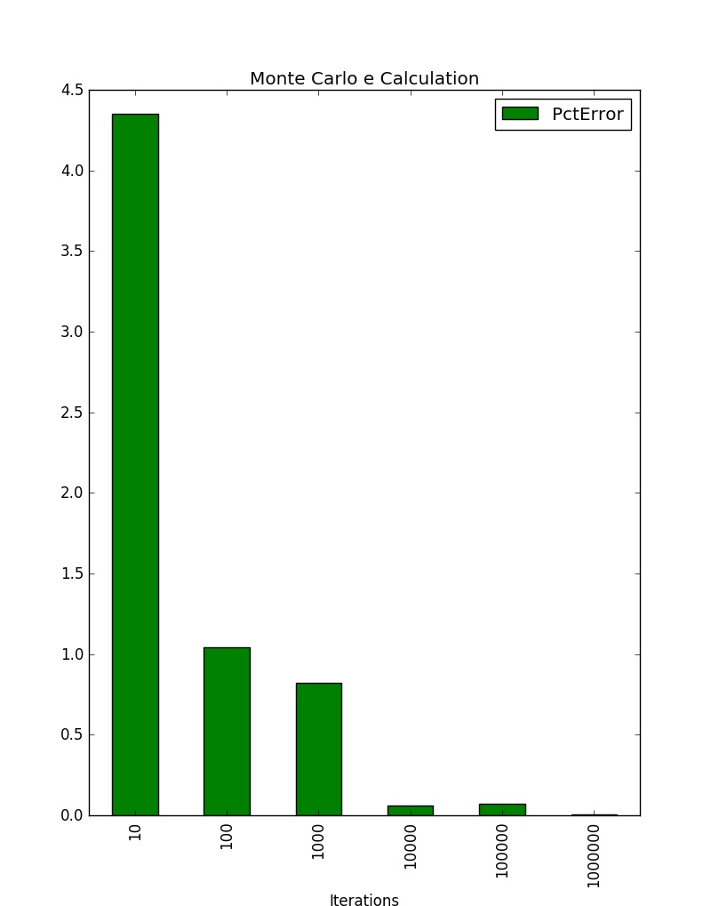
    frame.plot(x='Iterations', y='PctError', kind='bar', title='Monte Carlo e Calculation', color=['g'])
    plt.show()

Results

   Iterations  PctError
0          10  4.351345
1         100  1.040430
2        1000  0.819703
3       10000  0.058192
4      100000  0.072773
5     1000000  0.005512

Fire Ant Simulation

This last simulation is admittedly contrived and likely less than scientifically accurate.  The focus is on the Monte Carlo method.  However, I can say I have some first-hand experience with this model via ~20 years spent in Texas for under-grad work and various military assignments.  For those unfamiliar with fire ants - they are a uniquely offensive member of the animal kingdom.  They bite + sting and are extremely aggressive when disturbed.  Fire ants are in never-ending abundance in Texas.  On that note - I used some fire ant data from this Texas A&M website

This simulation is a model of a typical residential backyard and the fire ant population therein.  The question to be answered:  How long can I sit in my backyard until at least one fire ant is tearing me up?

Diagram of the model below:

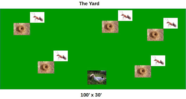
Rude awakening imminent

Model Assumptions

  • 100' x 30' = 3000 sq ft 'yard'
  • 5 ant mounds in the yard
  • 500K ants
  • Ant mounds are randomly distributed in yard
  • Ants are randomly distributed amongst the mounds.
  • All ants start the simulation at their home mound position.
  • Ants have 2 states in the model.  Foraging or attacking.
  • 1 human exists in the model.  The human is randomly positioned in the yard with the assumption they will not sit directly on a mound.  This assumption is a partial deviation from reality to ensure statistically interesting experiments.  I've personally sat on a fire ant mound (inadvertently).  I don't recall it being statistically interesting.
  • Ants move 3 inches/second, or 1 foot in 4 seconds.
  • Time steps in the model are 4 seconds
  • Ants on the move ('foraging') will randomly choose among 8 possible directions at each time step.  This provides the randomness of the model.
  • Ants on the move will stay the course in 1 direction for an entire time step (same direction for 1 foot/4 seconds)
  • Ants can't leave the boundaries of the yard.  An attempt to do so results in no movement for that time step.
  • Only 50% of the ant population makes a move in any given time step.  The rest are idle for that time step.
  • Once an ant gets within 1 foot of the human position, it starts attacking.  An attacking ant never leaves the 'attacking' state.  Again, I can attest from personal experience that this represents reality.
  • The simulation ends when at least 1 ant achieves the 'attacking' state.

Python Implementation

class Yard(object):
    length = 100 #3000 sq ft yard
    width = 30
    numMounds = 5
    numAnts = numMounds * 100000 #100K ants per mound
    pctAntsActive = .5 #percentage of the ants moving at any given time step
    
    def __init__(self):
        random.seed()
        self.__setMounds()
        self.__setAnts()
        self.__setHuman()
        
    def __setMounds(self): 
        self.moundPositions = []
        xlist = random.sample(range(0, Yard.length+1), Yard.numMounds)
        ylist = random.sample(range(0, Yard.width+1), Yard.numMounds)
        for i in range(Yard.numMounds):
            mound = (xlist[i], ylist[i])
            self.moundPositions.append(mound)
    
    def __setAnts(self):
        self.ants = []
        for _ in range(Yard.numAnts):
            mound = random.choice(self.moundPositions)
            self.ants.append(Ant(mound))
                
    def __setHuman(self):
        done = False
        while not done:
            x = random.randint(0, Yard.length)
            y = random.randint(0, Yard.width)
            if (x, y) not in self.moundPositions: 
                done = True
            else:
                pass
            
        self.humanPosition = (x, y)
    
    def clockTick(self):
        antsAttacking = 0
        activeAnts = random.sample(range(0, Yard.numAnts), int(Yard.numAnts*Yard.pctAntsActive))
        
        for ant in activeAnts:
            state = self.ants[ant].move(self.humanPosition)
            if state == 'attacking':
                antsAttacking += 1
                break
            else:
                pass
        
        return antsAttacking
Line 1:  Class definition of the "Yard"
Lines 2-6:  Class variables capturing some the model assumptions
Lines 8-12:  Class initializer which sets up the model.
Lines 14-20:  Function to randomly distribute the ant mounds in the yard.
Lines 22-26:  Function to create the ant objects and randomly distribute them among the mounds.
Lines 28-38:  Function to randomly position the human in the yard, but not on top of a mound.
Lines 40-52:  Main driver of the simulation.  Provides a four-second time step during which a random 50% distribution of ants make a one-foot move.  Function returns the number of ants that reached the 'attacking' state in that time step.

class Ant(object):
    __directions = ['NW', 'N', 'NE', 'E', 'SE', 'S', 'SW', 'W']
    
    def __init__(self, position):
        self.position = position
        self.state = 'foraging'
    
    def __checkAttack(self, humanPosition):
        distance = math.sqrt((self.position[0] - humanPosition[0])**2 + (self.position[1] - humanPosition[1])**2)
        if distance <= 1:
            return 'attacking'
        else:
            return 'foraging'
    
    def move(self, humanPosition):
        if self.state == 'foraging':
            direction = random.choice(Ant.__directions)
              
            if direction == 'NW':
                x = self.position[0] - 1
                y = self.position[1] + 1
            elif direction == 'N':
                x = self.position[0] 
                y = self.position[1] + 1
            elif direction == 'NE':
                x = self.position[0] + 1
                y = self.position[1] + 1
            elif direction == 'E':
                x = self.position[0] + 1
                y = self.position[1] 
            elif direction == 'SE':
                x = self.position[0] + 1
                y = self.position[1] - 1
            elif direction == 'S':
                x = self.position[0] 
                y = self.position[1] - 1
            elif direction == 'SW':
                x = self.position[0] - 1
                y = self.position[1] - 1
            elif direction == 'W':
                x = self.position[0] - 1
                y = self.position[1]
            else:
                pass
              
            if x >= 0 and x <= Yard.length and y >= 0 and y <= Yard.width:
                self.position = (x, y)
            else:
                pass
            self.state = self.__checkAttack(humanPosition)
        else:
            pass
        
        return self.state
Line 1:  Ant class definition
Line 2:  Class variable containing a list of the 8 different directions an ant can move
Lines 4-6:  Class initializer setting an ant's initial position and state.
Lines 8-13:  Private class function for determining if an ant is within 1 foot of the human's position.  If so, the ant's state is set to 'attacking.'
Lines 15-54:  Resets an ant position by 1 foot in a randomly chosen direction.  If the resulting position is outside of the yard boundaries, the ant remains stationary.  Returns the new state of the ant based on its new position.
def simulation(): 
    yard = Yard()
    seconds = 0
    numAttacking = 0
    
    while numAttacking == 0:
        numAttacking = yard.clockTick()
        seconds += 4
    
    return seconds
Lines 1-10:  Global function providing simulation driver.  Sets up the 'yard' and runs a clock until at least 1 ant is attacking the human.

if __name__ == '__main__': 
    simIters = [25,50,75,100]
    avg = {}
    
    for iters in simIters:
        tot = 0
        pool = mp.Pool()
        results = []
        for _ in range(iters):
            results.append(pool.apply_async(simulation))       
        pool.close()
        pool.join()
        for res in results:
            tot += res.get()
        avg[iters] = round(tot / iters)
        print(iters, avg[iters])
    
    
    frame = pd.DataFrame(data=list(avg.items()), columns=['Iterations', 'Seconds'])
    frame.sort_values(by='Iterations', inplace=True)
    frame.reset_index(inplace=True, drop=True)
    print(frame)
    frame.plot(x='Iterations', y='Seconds', kind='bar', title='Monte Carlo Fire Ant Attack Simulation', color=['r'])
    plt.show()        
Lines 2-16:  Sets up a loop that proceeds through 4 different iteration runs of the simulation (25,50,75,100) and creates a multiprocessing pool to run them.  Run time of each simulation is stored for its particular iteration count and then averaged.
Lines 19-24:  Sets up a pandas data frame with the results and display a bar graph.

Results

25 198
50 189
75 121
100 166
   Iterations  Seconds
0          25      198
1          50      189
2          75      121
3         100      166

These simulations maxed out all four cores on my machine for lengthy periods of time.  My guess would be if I were to run higher iteration counts, the attack time would settle somewhere around 150 seconds as that appears to be the trend with these 4 trials.


Source: https://github.com/joeywhelan/montecarlo

Copyright ©1993-2024 Joey E Whelan, All rights reserved.

Sunday, November 19, 2017

Crypto Digest Collisions


Summary

Proof-of-work is a critical component of the various crypto coin variants in use today.  In a nutshell, the blockchain algorithms that form the basis of crypto coins require participants to complete a provable amount of computation before a transaction can be added to the chain.  Partial hash collision is one such proof of work.

The post covers a toy implementation of partial hash collision.

Background

The basis for this proof-of-work method is hash digests.  An input string is processed through a cryptographically-strong function that outputs a fixed-length and unique hash value for that given input string.  Given a strong hash algorithm, it should be computationally unfeasible to find two input strings that create the same hash digest - also known as collision resistance.

Collisions on the full bit-length of a hash may be unfeasible, but collisions on a subset of the bits can be accomplished.  There are no known short-cuts to finding a collision but trial and error - submitting a different input string to a hash algorithm, over and over.  The typical partial hash collision method takes a string as input, concatenates a number to that string, then tests the high-order bits of the resulting hash.  If the necessary number of high-order bits are all 0, a solution has been found.

Example:  Say a given hash algorithm outputs a 10-bit hash and we want to find string with given input that results in the first 4 bits all equal to 0.  There are 2**10 total unique hashes available in this algorithm.  There are 2**6 hashes where the first 4 bits are 0.  In general, we would have to try 2**4 (16) inputs to the hash algorithm to find a solution.  Real world implementations deal with 160/256 bit hashes and collision lengths of >20 bits.

Implementation

Single Process

totalBits = 256  
collisionBits = 23 
mask = (1<<totalBits) - (1<<totalBits-collisionBits)
textInput = None

def singleProcessHash(text):
    count = 0    
    ti = time.time()
    
    while True:
        msg = text + ':' + str(count)
        dig = hashlib.sha256(msg.encode(encoding='utf_8', errors='strict')).hexdigest()
        res = int(dig,16) & mask
        if res == 0:
            break   
        count+=1
            
    print('Single-process run time: {:0.4f}'.format(time.time()-ti))
    print ('Message: ', msg)
    return msg
Lines 1-2:  Total bit length of the hash and the number of required high-order bits to be set to 0.  SHA-256 outputs a 256-bit hash.  For this example, the 23 high-order bits have to be 0 for a valid solution string.
Line 3:  Constucts a 256-bit mask with the 23 high-order bits set to 1.  All other bits are 0.
Lines 10-16: Brute-force loop that successively concats a number to the input text, hashes it thru SHA-256, and then does a bit-wise AND against the mask to test if the 23 high-order bits are all 0.  If the result isn't a partial collision, increment the counter and continue to loop.

Multiple Processes

def init(text):
    global textInput
    textInput = text
    
def findCollision(arg):
    global textInput
    msg = textInput + ':' + str(arg)
    hsh = hashlib.sha256(msg.encode(encoding='utf_8', errors='strict')).hexdigest()
    res = int(hsh,16) & mask
    if res == 0:
        return msg

def multiProcessHash(text):
    mult = 1
    numValues = 10**6
    chunkSize = math.ceil(numValues/mp.cpu_count())
    found = False
    msg = None
    ti = time.time()
   
    pool = mp.Pool(initializer=init, initargs=[text])
    while not found: 
        sample = range(numValues*(mult-1), numValues*mult)
        mult += 1
        results = pool.imap_unordered(findCollision, sample, chunkSize)
        for msg in results:
            if msg:
                pool.terminate()
                pool.join()
                found = True
                break

    print('Multi-process run time: {:0.4f}'.format(time.time()-ti))
    print('Message: ', msg)
    return msg
Lines 1-3:  Init function setting the text argument for each of the worker processes in the pool. Unfortunate aspect of Python, but use of globals is the most straight-forward way to accomplish this.
Lines 5-11:  Collision test function performed by each of the worker processes.
Line 15:  Variable to set up 1M values to be sent to the pool per iteration.
Line 16:  Chunk up those 1M test values evenly amongst the worker processes.  One worker per CPU.
Lines 21-31:  Set up the worker pool and loop through successive 1M value batches of samples until a partial collision is found.

Results

This was tested on a quad-core machine with hyper-threading (8 logical CPU's).
if __name__ == '__main__':
    singleProcessHash(string.ascii_uppercase)
    print()
    multiProcessHash(string.ascii_uppercase)  
Single-process run time: 18.9084
Message:  ABCDEFGHIJKLMNOPQRSTUVWXYZ:7201566

Multi-process run time: 6.7886
Message:  ABCDEFGHIJKLMNOPQRSTUVWXYZ:7201566


Copyright ©1993-2024 Joey E Whelan, All rights reserved.

Friday, September 8, 2017

AI-Driven Investing with Lending Club - Part 5: Ensembling


Summary

This is the fifth installment in the series I've written on my experience implementing a machine learning engine for selecting loans for investment from Lending Club.  In this article, I'll discuss and apply a couple techniques for combining the results of multiple classifiers.
There's quite a bit of literature out there on ensembling as it has been a popular (and winning) technique in Kaggle competitions.  In a nutshell, ensembling attempts to combine the strengths of multiple classifiers to produce a classifier that is better than its parts.

The simplest ensemble, and in fact has an out-of-box implementation in scikit-learn - VotingClassifier, is voting.  In 'hard' voting, the majority prediction from multiple classifiers is taken to be the final prediction.  In 'soft' voting, the probabilities from multiple classifiers are summed to come up with the final prediction.

A more complex ensembling technique is known as stacking (sometimes also referred to as 'blending').  In this model, classifiers are 'stacked' in levels.  The outputs of the classifiers in the lower levels become the inputs to the classifier(s) in the upper levels.

An interesting variation of stacking was developed for the Netflix Prize competition in 2009 and was in fact the 2nd place winner.  Feature-weighted Linear Stacking takes 'meta-features' and combines them via linear regression to a stacked model.  Video here from Joe Sill, a member of the 2nd place team, describing the technique.

Implementation

I decided to approach this with a Python class (Ensemble) that implements both voting and stacking.  I settled on four classifiers:  GBC, MLP, RBM, and SVD.  I ran all four through a grid-search to find a good parameter set for each classifier for my particular data set.

Below is some code that tests each classifier in isolation and prints out a Pearson correlation matrix for the four classifiers.  Good classification performance per classifier and low-correlation between classifiers are goals for an ensemble.
        pool = mp.Pool(processes=mp.cpu_count())
        results = []

        for name, clf in self.estimators.items():
            try:
                self.estimators[name] = joblib.load('./models/' + name + '.pkl')
            except FileNotFoundError:  
                logging.debug('{} not pickled'.format(name))    
                results.append(pool.apply_async(lvl1_fit, args=(clf, name, features_train, labels_train)))           
           
        pool.close()
        pool.join() 
        for result in results:
            item = result.get()
            name = item['name']
            self.estimators[name] = item['fittedclf']
        
        #Print confusion matrix and score for each clf.  
        corr_list = []
        clf_list = []
        for name, clf in self.estimators.items():
            preds = clf.predict(features_test)
            self.confusion_matrix(name, labels_test, preds)
            print()
            self.classification_report(name, labels_test, preds)
            corr_list.append((name, preds))
            clf_list.append(name)
        
        #Print a matrix of correlations between clfs
        frame = pd.DataFrame(index=clf_list, columns=clf_list)
    
        for pair in itertools.combinations(corr_list,2):
            res = pearsonr(pair[0][1],pair[1][1])[0]
            frame[pair[0][0]][pair[1][0]] = res
            frame[pair[1][0]][pair[0][0]] = res
        frame['mean'] = frame.mean(skipna=True,axis=1)
        pd.options.display.width = 180
        print('Correlation Matrix')
        print(frame) 

Lines 1-16: Load up the fitted classifiers.  'estimators' is an OrderedDict of scikit-learn classifier objects.  If the fitted classifiers have already been cached to disk, use that.  Otherwise, fit them from scratch on the training set in a multiprocessing pool.
Lines 18-27:  Generate predictions for each classifier for the test set, then print a confusion matrix and classification report for each.
Lines 29-39:  Generate the Pearson correlation between each pair of classifiers and then organize the results in a matrix.

Excerpt of the output below:
svd Confusion Matrix (66392 samples): 
[[ 8599  4654]
 [22715 30424]]

svd Classification Report
             precision    recall  f1-score   support

    Default       0.27      0.65      0.39     13253
       Paid       0.87      0.57      0.69     53139

avg / total       0.75      0.59      0.63     66392

Correlation Matrix
          gbc       mlp       rbm       svd      mean
gbc       NaN  0.746548  0.603429  0.532055  0.627344
mlp  0.746548       NaN  0.516596  0.538988  0.600711
rbm  0.603429  0.516596       NaN  0.408401  0.509475
svd  0.532055  0.538988  0.408401       NaN  0.493148

Voting

The voting portion is quite simple as it is simply a wrapper around the out-of-box implementation from scikit-learn.

Fitting of the voting classifier below:
        try:
            self.voteclf = joblib.load('./models/voteclf.pkl')
        except FileNotFoundError: 
            ti = time() 
            self.voteclf = VotingClassifier(estimators=list(self.estimators.items()), voting='soft',n_jobs=-1)      
            self.voteclf.fit(features_train, labels_train)
            joblib.dump(self.voteclf, './models/voteclf.pkl') #cache the fitted model to disk
        logging.debug('Exiting __fit_vote()')
Lines 1-9:  If the voting classifier has already been fitted and cached to disk, load it.  Otherwise, fit it from scratch and dump the fitted model to disk.

Prediction with the voting classifier below:
preds = self.__predict_with_threshold(self.voteclf, features)

def __predict_with_threshold(self, clf, features):
        ti = time()
        predictions = Ensemble.__custom_predict(clf.predict_proba(features)[:, MINORITY_POS], \
                                                clf.predict(features), self.threshold)
        return predictions

__custom_predict = np.vectorize(vfunc, otypes=[np.int])

def vfunc(probability, prediction, threshold):
    if probability >= threshold:
        return MINORITY_CLASS
    else:
        return prediction
Line 1:  Pass the fitted voting classifier to a custom predict function that operates with thresholds.
Lines 3-15:  Custom prediction function that uses a threshold to decide whether the minority class should be chosen as the prediction.  This is a method to deal with unbalanced classes.

Stacking

The stacking implementation is significantly more complex.  Fitting, for example, requires fitting of each of the four 1st level classifiers and then fitting each of them in K-Fold cross-validation to generate the training data for the 2nd level classifier.  I'm using an unbalanced data set from Lending Club that has over 600K records.  Balancing that takes its size to a ~1M records.  Fitting on data sets of this size mandates use of multiprocessing and caching of the fitted classifiers to disk.

        pool = mp.Pool(processes=mp.cpu_count())
        results = [] #array for holding the result objects from the pool processes
        
        #fit 1st level estimators with a multiprocessing pool of workers
        for name, clf in self.estimators.items():
            try:
                self.estimators[name] = joblib.load('./models/' + name + '.pkl')
            except FileNotFoundError:  
                logging.debug('Level 1: {} not pickled'.format(name))    
                results.append(pool.apply_async(lvl1_fit, args=(clf, name, features_train, labels_train)))           
           
        pool.close()
        pool.join() 
       
        for result in results:
            item = result.get()
            name = item['name']
            self.estimators[name] = item['fittedclf'] #reassign a fitted clf to the estimator dictionary
        
        #fit 2nd level estimator with a multiprocessing pool of workers that perform a k-fold cross-val of 
        #training data
        pool = mp.Pool(processes=mp.cpu_count())
        del results[:]
        try:
            self.lrc = joblib.load('./models/lrc.pkl') #try to load the 2nd level estimator from disk
        except FileNotFoundError: #2nd level estimator not fitted yet
            logging.debug('Level 2: LRC not pickled') 
            folds = list(StratifiedKFold(n_splits=5).split(features_train, labels_train)) 
            #define a frame for holding the k-fold test results of the 1st level classifiers
            lvl2_frame = pd.DataFrame(index=range(0,len(features_train)), 
                                      columns=list(self.estimators.keys()))  
            lvl2_frame[LABEL_COL] = labels_train  
             
            #launch multiprocessing pool workers (1 per fold) that fit 1st level classifers and perform
            #predictions that become the training data for the 2nd level classifier (Logistic Regression)   
            for name,clf in self.estimators.items():
                fold = 1
                for train_idx, test_idx in folds:
                    X_train, X_test = features_train[train_idx], features_train[test_idx]
                    Y_train = labels_train[train_idx]
                    col_loc = lvl2_frame.columns.get_loc(name)
                    results.append(pool.apply_async(lvl2_fit, args=(clf, name, fold, test_idx, \
                                                                    col_loc, X_train, Y_train, X_test)))
                    fold = fold + 1
            pool.close()
            pool.join() 
           
            #fetch worker results and put them into a frame that will be used to train a 2nd Level/Logistic
            #regression classifier
            for result in results:
                item = result.get()
                name = item['name']
                test_idx = item['test_idx']
                col_loc = item['col_loc']
                preds = item['preds']
                lvl2_frame.iloc[test_idx, col_loc] = preds

            self.lrc = LogisticRegression(C=2.0)
            ti = time()
            X = lvl2_frame.drop(LABEL_COL, axis=1).values
            Y = lvl2_frame[LABEL_COL].values
            self.lrc.fit(X, Y)     
            logging.debug('LRC fit time: {:0.4f}'.format(time()-ti))
            joblib.dump(self.lrc, './models/lrc.pkl')  #cache the Logistical Regressor to disk

def lvl1_fit(clf, name, features_train, labels_train):
    logging.debug('Entering lvl1_fit() {}'.format(name))
    ti = time()
    fittedclf = clf.fit(features_train, labels_train)
    logging.debug('{} fit time: {:0.4f}'.format(name, time()-ti))
    joblib.dump(fittedclf, './models/' + name + '.pkl') #cache the fitted model to disk
    logging.debug('Exiting lvl1_fit() {}'.format(name))
    return {'name': name, 'fittedclf': fittedclf}

def lvl2_fit(clf, name, fold, test_idx, col_loc, features_train, labels_train, features_test):  
    logging.debug('Entering lvl2_fit() {} fold {}'.format(name, fold))
    ti = time()
    clf.fit(features_train, labels_train)
    logging.debug('{} fold {} fit time: {:0.4f}'.format(name, fold, time()-ti))
    preds = clf.predict_proba(features_test)[:, MINORITY_POS]
    logging.debug('Exiting lvl2_fit() {} fold {}'.format(name, fold))
    return {'name': name, 'test_idx' : test_idx, 'col_loc' : col_loc, 'preds' : preds}
Lines 1-18:  Attempt to load fitted classifiers from disk.  If they don't exist, use a pool of workers to fit each classifier to the full training set.
Lines 20-56:  With K-Fold (5 folds) cross validation, fit each of the classifiers and then generate predictions with the test set in that fold.  Save the predictions to a data frame.
Lines 58-64:  Fit the 2nd level classifier (Logistic Regression) to the predictions from the 1st level classifiers.  Dump the fitted Logistic classifier to disk.
Lines 66-73:  Function for fitting the 1st level classifiers and dumping them to disk.
Lines 75-82:  Function called within the K-folding for fitting 1st level classifiers and generating predictions to use to train the 2nd level classifier.

Generating predictions from the stacked ensemble requires running the features through all of the 1st level classifiers and then sending their output (predictions) to the 2nd level classifier - Logistic Regression.
 def __predict_stack(self, features):
        lvl1_frame = pd.DataFrame()
        #1st level predictions
        for name, clf in self.estimators.items():
            lvl1_frame[name] = clf.predict_proba(features)[:, MINORITY_POS]
            
        #2nd level predictions
        preds = self.__predict_with_threshold(self.lrc, lvl1_frame.values)
   
        return preds

Source:  https://github.com/joeywhelan/Ensemble/

Copyright ©1993-2024 Joey E Whelan, All rights reserved.

Thursday, June 8, 2017

Secure DNS Conversion


Summary


I'll be discussing a little distraction I was working on lately in this article.  There are a large number of articles out there about the inherent insecurity of DNS.  Your requests/responses are clear text that runs (predominantly) over UDP.  Every ISP, DNS provider, etc basically has goods on whatever Internet sites you may visit.

In a few lines of code (~200), I show one way to keep your DNS traffic private.  Part 1 hinges on Google's HTTPS DNS services.  I convert the UDP DNS request into an HTTPS request to Google for an encrypted DNS request/response system.  To raise this to another level of paranoia (for those that don't even trust Google with their DNS traffic), I show how to tunnel those requests to Google through Tor.

I made little attempt to faithfully follow the DNS RFC in this implementation.  Just wasn't necessary for my limited use-case.

Implementation - Part 1

Below is a diagram of the overall architecture I was looking for.  I use a local caching DNS server for my own network.  I reconfigure that DNS server to send all of its requests to my DNS converter that translates DNS UDP requests into HTTP calls to Google's DNS over HTTPS service.


Python Implementation


cfgParser = configparser.ConfigParser()
cfgParser.optionxform = str
cfgParser.read('sdns.cfg')  
host = cfgParser.get('ConfigData', 'host')
port = int(cfgParser.get('ConfigData', 'port'))
server = socketserver.UDPServer((host, port), DNSHandler)
server.serve_forever()
Lines 1-5:  Read the host IP address and Port for the new DNS converter/forwarder.  DNS runs on port 53 typically.
Lines 8-9:  Start a UDP server on that IP address and port.  DNSHandler is a class that contains the code to process the DNS request and generate the response.
class DNSHandler(socketserver.BaseRequestHandler):
    
    def handle(self):
        data = self.request[0]
        socket = self.request[1]
        response = self.__createResponse(data)
        socket.sendto(response, self.client_address)
Lines 3-7:  Main code body.  Accepts the request, processes it, and sends out the response.

    def __createResponse(self, data):
        tid = data[0:2] #transaction id
        opcode = data[2] & 0b01111000   #data[2] is the flags field. bits 2-5 is the opcode  
        name, queryType, question = self.__processQuestion(data[12:]) 
        
        if opcode == 0 and queryType == '1':  #RFC departure.  Only processing standard queries (0) and 'A' query types.  
            flags, numbers, records = self.__getRecords(name)
            response = tid + flags + numbers + question + records
        else:
            #qr (response), recursion desired, recursion avail bits set.  set the rcode to 'not implemented'
            flags = ((0b100000011000 << 4) | 4).to_bytes(2, byteorder='big') 
            numbers = (0).to_bytes(8, byteorder='big')
            response = tid + flags + numbers
 
        return response
Lines 2-3:  Parse out the DNS transaction ID and flag field from the request.
Line 4:  Send the rest of the DNS request to another function for parsing out the question.
Lines 6-8:  If it's a DNS request I chose to implement, standard 'A' type,  process it.
Lines 10-13:  If it's not a request I implemented, return a DNS error.

    def __processQuestion(self, quesData):
        i = 0
        name = ''
        
        while True:
            count = int.from_bytes(quesData[i:i+1], byteorder='big')
            i = i+1
            if count == 0:
                break
            else:
                name = name + str(quesData[i:i+count],'utf-8') + '.'
                i = i + count
            
        name = name[:-1]
        queryType = str(int.from_bytes(quesData[i:i+2], byteorder='big'))
        question = quesData[0:i+4]
   
        return name, queryType, question
Lines 5-12:  Loop thru the labels in the DNS question (it has a specific format, see RFC).
Lines 14-16: Set up 3 return variables with the domain name in question, query type, and the entire question byte array (for the response to be sent later).

    def __getRecords(self, name): 
        payload = {'name' : name, 'type' : '1'}
        data = requests.get(GOOGLE_DNS, params=payload).json()
   
        flags = self.__getFlags(data)
        records = bytes(0)
        count = 0
        if 'Answer' in data:
            for answer in data['Answer']:
                if answer['type'] == 1:
                    count = count + 1
                    name = (0xc00c).to_bytes(2, byteorder='big') #RFC departure.  Hard-coded offset to domain name in initial question.
                    rectype = (1).to_bytes(2, byteorder='big')
                    classtype = (1).to_bytes(2, byteorder='big')
                    ttl = answer['TTL'].to_bytes(4, byteorder='big')
                    length = (4).to_bytes(2, byteorder='big') #4 byte IP addresses only
                    quad = list(map(int, answer['data'].split('.')))
                    res = bytes(0)
                    for i in quad:
                        res = res + i.to_bytes(1, byteorder='big')
                    records = records + name + rectype + classtype + ttl + length + res
        
        nques = (1).to_bytes(2, byteorder='big') #hard coded to 1
        nans = (count).to_bytes(2, byteorder='big')
        nath = (0).to_bytes(2, byteorder='big')    #hard coded to 0
        nadd = (0).to_bytes(2, byteorder='big') #hard coded to 0
        numbers = nques + nans + nath + nadd
     
        return flags, numbers, records
Lines 2-3:  Send the DNS request to Google's HTTPS service.
Line 5:  Construct the flags field for the response based on the request flags field.
Lines 8-21:  Construct the Return Records fields for the response from the JSON response from Google's DNS/HTTPS service.
Lines 23-27:  Construct the number of records field for the response.
    def __getFlags(self, data):
        flags = 0b100000 #qr=1, opcode=0000, aa=0
        flags = (flags << 1) | data['TC'] #set tc bit
        flags = (flags << 1) | data['RD'] #set rd bit
        flags = (flags << 1) | data['RA'] #set ra bit
        flags = flags << 1 #One zero
        flags = (flags << 1) | data['AD'] #set ad bit
        flags = (flags << 1) | data['CD'] #set cd bit
        flags = ((flags << 4) | data['Status']).to_bytes(2, byteorder='big') 
 
        return flags
Lines 2-9:  Construct the flags field of the DNS response based on the JSON response from Google (and some hard-coded values).

Implementation - Part 2

Now to prevent even Google to track your DNS activity, we can send all this HTTPS traffic on a world-wide trip through the Tor network.  You need to set up a local Tor controller instance and then add the lines of code below to direct the HTTPS request through that network.  Here's an excellent explanation for that.


Python Implementation


PROXIES = {'http':  'socks5://127.0.0.1:9050',
           'https': 'socks5://127.0.0.1:9050'} 

data = requests.get(GOOGLE_DNS, params=payload, proxies=PROXIES).json()
Lines 1-2:  Tor uses port 9050 as its local SOCKS port.
Line 4: Simply modify the HTTPS Get to Google (from __getRecords()) with these proxies.
def renew():
    with Controller.from_port(port = 9051) as controller:
        controller.authenticate(password="test")
        controller.signal(Signal.NEWNYM)

  
scheduler = BackgroundScheduler()
scheduler.add_job(renew, 'interval', hours=1)
scheduler.start()
Lines 1-4:  For some extra security, signal your Tor controller to change its IP address periodically.
Lines 7-9:  Set that change interval with a scheduler.

Summary

This was a fairly simplistic DNS server implementation in Python.  I didn't attempt to implement the full RFC as it's not necessary for my use case.  You get secure DNS traffic from this but at the price of latency.  The HTTPS conversion and Tor overhead equates to a factor of 10 increase in DNS latency (the vast majority of that is attributable to Tor).  I don't find it noticeable though for my use.

Full source code here.

Copyright ©1993-2024 Joey E Whelan, All rights reserved.

Sunday, February 26, 2017

IoT Data Pipeline - Part 3: Kafka Integration


Summary

In this post I'll scale up the architecture by simulating multiple IoT devices and then consolidate the resulting data stream into Apache Kafka.

IoT Data Pipeline - Part 2: Node/Java Crypto Interop
IoT Data Pipeline - Part 3:  Kafka Integration

Implementation

Diagram below depicting the overall set up I'm trying to achieve here.  I wanted to scale up the number of devices generating data streams to the IoT cloud and then consolidate them into a scalable streaming architecture - which is Kafka.  

As mentioned in the first post, this exercise is somewhat contrived.  I scaled up data generators by creating device simulators.  On the receiving side of the IoT cloud, multiple REST clients poll for data (1 per device) and then write into Kafka.

Lower level diagram of the code below:


Node.js - Device Server Code Modifications


var devices = [];
for (var i=0; i < properties.deviceCount; i++) {
 devices.push('pws_' + i);
}

function rand(min, max) {
 return Math.random() * (max - min) + min + 1;
}
function randomize(data) {
 for (var prop in data){
  if (data.hasOwnProperty(prop)) {
   rn = rand(-.5,.5);
   data[prop] = (data[prop] * rn).toFixed(2);
  }
 }
 return data;
}

function thingspace(requrl) {
 var query = url.parse(requrl, true).query;
 var wx_data = {'windspeedmph' : query.windspeedmph, 'solarradiation' : query.solarradiation};
 
 var options = {
   host : 'thingspace.io',
   port : '443',
   headers: {'Content-Type' : 'application/json'},
   method : 'POST'
 };
 
 async.map(devices, function(device, callback){
  var iv = crypto.randomBytes(16);
  var cipher = crypto.createCipheriv('aes-256-cbc', key, iv);
  wx_data = randomize(wx_data);
  wx_data.id = device;
  var cipherText = cipher.update(JSON.stringify(wx_data), 'utf8','hex') + cipher.final('hex');
  options.path = '/dweet/for/' + device;
  
  var retVal = '';
  var req = https.request(options, function(res) {
   res.on('data', function(chunk) {
    retVal += chunk;
   });
   res.on('end', function() {
    retVal = JSON.parse(retVal);
    callback(null, retVal.this);
   });
  });

  req.on('error', function(err1) {
   logger.error('File: main.js, Method: thingspace(), Message err1: ', err1.message);
   callback(err1, null);
  });
  req.write(JSON.stringify({'iv': iv.toString('base64'), 'mesg' : cipherText}));
  req.end(); 
 }, 
 function (err, results){
  if (err) {
   logger.error('File: main.js, Method: thingspace(), Message err: ', err.message);
  }
  else {
   logger.debug('Exiting - File: main.js, Method: thingspace()');
  }
 });
}


function handler(req, res) {
 wunderground(req.url, res);
 thingspace(req.url);
}

var httpServer = http.createServer(handler).listen(9080);
logger.debug('File: main.js, Listening on port 9080');
Lines 1-4:  Set up an array of simulated IoT devices.
Lines 6-17:  Couple functions to generate random data metrics to the simulated devices.  Data from the one real device is fed into these functions and random data for the simulators is generated from that.
Line 21:  The two metrics being sent from the devices are solar radiation and wind speed.
Lines 30-47:  This is where the device simulation happens.  Using the Async module, send out multiple HTTP REST requests (1 per simulated device) to the IoT cloud.

Java - Custom JSON Serializer/Deserializer for Kafka

Kafka operates with byte arrays.  It has a built-in serializer for Strings.  If you want pass anything other than that, you have to roll your own.

public class JSONSerializer implements Serializer {
 @Override
  public void close() {
  
  }
 
 @Override
  public void configure(Map arg0, boolean arg1) {
  
  }
 
 @Override
 public byte[] serialize(String s, JSONObject json) {
  byte[] byteArr = null;
  
     try {
      ByteArrayOutputStream out_byte = new ByteArrayOutputStream();
      ObjectOutputStream out_object = new ObjectOutputStream(out_byte);
      out_object.writeObject(json);
      byteArr = out_byte.toByteArray();
     }
     catch (Exception e) {
      e.printStackTrace();
     }
     
     return byteArr;
 }
}
Lines 17-20:  Convert the JSON object into a byte array.

public class JSONDeserializer implements Deserializer {
 @Override
  public void close() {
  
  }
 
 @Override
  public void configure(Map arg0, boolean arg1) {
  
  }
 
 @Override
 public JSONObject deserialize(String s, byte[] bytes) {
  JSONObject json = null;
  
  try {
   ByteArrayInputStream bIstream= new ByteArrayInputStream(bytes);
   ObjectInputStream in = new ObjectInputStream(bIstream);
   json = (JSONObject) in.readObject();
  }
  catch (Exception e) {
   e.printStackTrace();
  }
  return json;
 }
}
Lines 17-19:  Convert a byte array into a JSON object.

Java - REST Clients/Kafka Producer


public class DweetProducer implements Runnable {

 private static final Logger logger = LogManager.getLogger(DweetProducer.class);
 private static final String propFile = "pwskafka.properties";
 private static final String dweetUri = "https://thingspace.io";
 private static final String streamPath = "/listen/for/dweets/from";
 private static byte[] salt;
 private static String password;
 private static String topic;
 private static String bootstrap;
 private static Producer producer;
 private String device;
 
 static {
  try {
   FileInputStream fis = new FileInputStream(propFile);
   Properties props = new Properties();
   props.load(fis);
   fis.close();
   salt = props.getProperty("salt").getBytes();
   password = props.getProperty("password");
   bootstrap = props.getProperty("bootstrap");
   topic = props.getProperty("topic");
   props.clear();
      props.put("bootstrap.servers", DweetProducer.bootstrap); 
      props.put("key.serializer", "org.apache.kafka.common.serialization.StringSerializer");
      props.put("value.serializer", "pwskafka.JSONSerializer");
      producer = new KafkaProducer(props);
  }
  catch (Exception e) {
   logger.error(e);
   System.exit(1);
  }
 }
 
 public DweetProducer(String device) {
  this.device = device;
  logger.debug("Producer for " + device  + " starting.");
 }
  
 private JSONObject decryptDweet(byte[] iv, String cipherText) throws GeneralSecurityException, 
 UnsupportedEncodingException, ParseException  {
  KeySpec spec = new PBEKeySpec(DweetProducer.password.toCharArray(), DweetProducer.salt, 100000, 256);
  SecretKeyFactory f = SecretKeyFactory.getInstance("PBKDF2WithHmacSHA256");
  SecretKey tmp = f.generateSecret(spec);
  SecretKey key = new SecretKeySpec(tmp.getEncoded(), "AES");
  
  Cipher cipher = Cipher.getInstance("AES/CBC/PKCS5Padding");
        cipher.init(Cipher.DECRYPT_MODE, key,  new IvParameterSpec(iv));
        String val = new String(cipher.doFinal(DatatypeConverter.parseHexBinary(cipherText)), "UTF-8");
        JSONParser parser = new JSONParser();
        return (JSONObject) parser.parse(val); 
 }
 
 public void run() { 
  JSONObject dweet = null;
  Client client = ClientBuilder.newClient();
  WebTarget target = client.target(dweetUri).path(streamPath).path(this.device);
  Response response =  target.request(MediaType.APPLICATION_JSON).get(Response.class);
  ChunkedInput chunkedInput =
          response.readEntity(new GenericType>() {});
  String chunk;
  JSONParser parser = new JSONParser();
  
  while ((chunk = chunkedInput.read()) != null) {
      if (!chunk.chars().allMatch( Character::isDigit )) {
       try {
        chunk = (String) parser.parse(chunk);
        JSONObject obj = (JSONObject) parser.parse(chunk);
        JSONObject content = (JSONObject) obj.get("content");
        byte[] iv = DatatypeConverter.parseBase64Binary((String) content.get("iv"));
     String cipherText = (String) content.get("mesg");
     dweet = decryptDweet(iv, cipherText);
     DweetProducer.producer.send(new ProducerRecord(DweetProducer.topic, this.device, dweet));
     logger.debug(dweet);
       }
       catch (Exception e) {
        logger.error(e);
       }
      }
  }
 }
 
 public static void main(String[] args) { 
  if (args != null && args.length == 2) {
   int startDeviceNum = Integer.parseInt(args[0]);
   int endDeviceNum = Integer.parseInt(args[1]);
   if (startDeviceNum > endDeviceNum) {
    logger.error("Usage:  arg 1: starting device number, arg 2: ending device number");
    System.exit(1);
   }
   ExecutorService pool;
   int cores = Runtime.getRuntime().availableProcessors();
   pool = Executors.newFixedThreadPool(cores);
   String device = null;
   
   for (int i = startDeviceNum; i <= endDeviceNum; i++){
    device = "pws_" + i;
    pool.execute(new DweetProducer(device));
   }
   pool.shutdown();
  }
  else {
   logger.error("Usage:  arg 1: starting device number, arg 2: ending device number");
   System.exit(1);
  }
 }

}
Line 1:  Setting up a multi-threaded class.
Line 12:  The Kafka Producer class is thread-safe, so we only need 1 instance that can be shared by all the threads.
Lines 14-34:  Load all the configuration variables from a properties file and create the Producer.  Line 27:  Tell the Producer how to serialize JSON objects using the customer serializer.
Lines 41-53:  AES decryption routine.  Same code as was discussed in Part 2.
Lines 55-82:  Thread code for HTTP clients.  Each client is doing HTTP chunked input using the IoT cloud's streaming interface.  This was discussed in Part 1.  Line 74:  Send the device data (dweet) to Kafka.
Lines 84-107:  Using the Java ExecutorService, set up a thread pool using all available cores.  Each thread will be executing a HTTP client with a common Kafka producer.

Test Kafka Consumer

public class DweetConsumer {
 
 public static void main(String[] args) throws Exception{
    String topicName = "pws_metrics";
    
    Properties props = new Properties();
    props.put("bootstrap.servers", "webserv3:9092"); 
    props.put("group.id", "group_01");
    props.put("key.deserializer", "org.apache.kafka.common.serialization.StringDeserializer");
    props.put("value.deserializer", "pwskafka.JSONDeserializer");
    props.put("enable.auto.commit", "true");
    props.put("auto.commit.interval.ms", "1000");
    props.put("session.timeout.ms", "30000");
    
    KafkaConsumer consumer = new KafkaConsumer<>(props);
    consumer.subscribe(Arrays.asList(topicName));
    
    while (true) {
     ConsumerRecords records = consumer.poll(100);
     for (ConsumerRecord record : records) {
      System.out.println("Received: " + record.key() + " " + record.value());
     }
    }
   
  }
}
Line 10:  Tell the Consumer how deserialize the incoming byte array back in to a JSON object.
Lines 15-16:  Set up a Kafka Consumer and subscribe to the IoT topic the Producer is creating records for.
Lines 18-23:  Poll for incoming records and print them to console.

Copyright ©1993-2024 Joey E Whelan, All rights reserved.

Sunday, January 29, 2017

IoT Data Pipeline - Part 2: Node/Java Crypto Interop


Summary

I wasn't planning on dedicating an entire post to encryption, but this task proved to be enough of a pain that I decided it was justified.  Maybe this will help others bypass that pain.

This project developed into a mixed-language solution:  Node on the server side (simulated device) and Java on the client/analytics side.  Getting Node-side encryption to work with the Java-side decryption is focus of this post.

IoT Data Pipeline - Part 2: Node/Java Crypto Interop
IoT Data Pipeline - Part 3: Kafka Integration

Implementation

Below is a diagram depicting the high-level steps I used to get a functioning encryption system between Node and Java.  There are likely other ways to go about this, but this is what worked for me.

Node Server Code

I've highlighted the crypto changes I made from original server code in the first blog post.
var key = crypto.pbkdf2Sync(properties.password, properties.salt, 100000, 32, 'sha256');

function thingspace(requrl) {
 var query = url.parse(requrl, true).query;
 var wx_data = {'tempf' : query.tempf, 'humidity': query.humidity, 
   'winddir' : query.winddir, 'windspeedmph' : query.windspeedmph, 
   'rainin' : query.rainin, 'solarradiation' : query.solarradiation};
 var options = {
   host : 'thingspace.io',
   port : '443',
   path : '/dweet/for/' + properties.device,
   headers: {'Content-Type' : 'application/json'},
   method : 'POST'
 };
 
 var iv = crypto.randomBytes(16);
 var cipher = crypto.createCipheriv('aes-256-cbc', key, iv);
 var cipherText = cipher.update(JSON.stringify(wx_data), 'utf8','hex') + cipher.final('hex');
 
 var retVal = '';
 var req = https.request(options, function(res) {
  res.on('data', function(chunk) {
   retVal += chunk;
  });
  res.on('end', function() {
   retVal = JSON.parse(retVal);
   logger.debug('Exiting - File: main.js, Method:thingspace()', retVal.this);
  });
 });

 req.on('error', function(err1) {
  logger.error('File: main.js, Method: thingspace(), Message err1: ', err1.message);
 });
 req.write(JSON.stringify({'iv': iv.toString('base64'), 'mesg' : cipherText}));
 req.end();
}
Line 1:  Create a secure 256-bit key with PBKDF2.
Line 16:  Generate a random 128-bit initialization vector.  Buffer of 16 bytes.
Line 17-18:  Encrypt the weather data (stringified JSON object) with AES 256 with UTF-8 input encoding and hex output encoding.
Line 34:  Encode the IV bytes into a Base64 string.  Then, put it and the encrypted message inside a JSON object.  Finally, stringify that object and send it out in the body of an HTTP POST.  There's no harm in sending the IV along with the encrypted message.

Java Client Code

Similar to the node server sample code, I've highlighted the crypto-interesting areas.

 public Object getDweet(String device) {
  
  Object dweet = null;
  Client client = ClientBuilder.newClient();
  WebTarget target = client.target(dweetUri).path(getPath).path(device);
  Response response =  target.request(MediaType.APPLICATION_JSON).get(Response.class);
  
  if(response.getStatus() == 200) {
   String message = response.readEntity(String.class);
   JSONParser parser = new JSONParser();
   try {
    JSONObject obj = (JSONObject) parser.parse(message);
    JSONObject item = (JSONObject) ((JSONArray)obj.get("with")).get(0);
    JSONObject content = (JSONObject)item.get("content");
    byte[] iv = DatatypeConverter.parseBase64Binary((String) content.get("iv"));
    String cipherText = (String) content.get("mesg");
    dweet = decryptDweet(iv, cipherText);
   }
   catch (Exception e) {
    e.printStackTrace();
   }
  }  
  return dweet;
 }

 private Object decryptDweet(byte[] iv, String cipherText) throws GeneralSecurityException, 
 UnsupportedEncodingException, ParseException  {
  KeySpec spec = new PBEKeySpec(this.password.toCharArray(), this.salt, 100000, 256);
  SecretKeyFactory f = SecretKeyFactory.getInstance("PBKDF2WithHmacSHA256");
  SecretKey tmp = f.generateSecret(spec);
  SecretKey key = new SecretKeySpec(tmp.getEncoded(), "AES");
  
  Cipher cipher = Cipher.getInstance("AES/CBC/PKCS5Padding");
                cipher.init(Cipher.DECRYPT_MODE, key,  new IvParameterSpec(iv));
                String val = new String(cipher.doFinal(DatatypeConverter.parseHexBinary(cipherText)), "UTF-8");
                JSONParser parser = new JSONParser();
                return parser.parse(val);
 }
Lines 12-14: Parse out the JSON object within the HTTP response body.  I'm using the json.simple toolkit for this.
Line 15:  Decode the Base64 string-encoded IV back to a byte array.
Lines 16-17:  Pass the encrypted text and and IV as input to a decrypt function.
Lines 28-31:  Generate the PBKDF2 secret key.
Lines 33-34:  Set up the AES decrypt cipher, with the IV.
Line 35:  Decrypt the message with hex input and UTF-8 output.
Lines 36-37:  Return the decrypted message as a JSON object.

Copyright ©1993-2024 Joey E Whelan, All rights reserved.

Thursday, January 19, 2017

IoT Data Pipeline - Part 1: Device Set up


Summary

In this post I'll describe my beginning steps in building a IoT data pipeline.  The scenario is somewhat contrived, but it uses infrastructure I have combined with no-cost interfaces.  The IoT 'device' in this scenario is a Personal Weather Station (PWS) I have installed on my place.  It's made by Ambient Weather - Model WS-1400-IP.  I integrated that to a cloud storage service from Verizon with a bit of Node.js code.

IoT Data Pipeline - Part 1: Device Set up
IoT Data Pipeline - Part 2: Node/Java Crypto Interop
IoT Data Pipeline - Part 3: Kafka Integration

Device

The 'IoT' device I used was an existing WS-1400-IP PWS I installed last year.  The PWS has an outdoor unit with various sensors for temperature, wind speed/direction, precipitation, etc.  It's solar-powered.  There's an additional indoor unit with a wireless receiver, Ethernet port, and firmware to run a web stack.  The indoor unit communicates with the outdoor via wireless transmissions.  Sensor data is then output to an internal HTTP server that can be accessed via the Ethernet interface. Optionally, the firmware supports transmission of the data to the Wunderground network.

Below is a picture of the PWS, photo-bombed by my mules.


The firmware that was installed on my PWS left much to be desired as far as access to the raw data stream.  By default, the PWS can send an HTTP GET with the data as a query string to Wunderground.  Unfortunately, that destination address is hard-coded into the firmware - making it impossible to redirect it for my own use.  There are various folks out there that have hacked around that limitation either by issuing commands directly to the firmware or with IP routing redirects - examples here.  I ended up putting another firmware load on the unit, not necessarily supported for my model, that provided a web interface for directing output to somewhere other than Wunderground.

Implementation

Now with access to the PWS data stream, I was in a position to do something with it.  I decided to build a simple Node.js server for accepting data from the PWS.  The PWS sends its data in the clear as query string via HTTP Get.  That plaintext data includes your Wunderground username and password - which is less than desirable, but it is what it is.  

The Node server in this case simulates a device that can then communicate to Verizon's IoT infrastructure.  Verizon ThingSpace has a freely available (as of now) REST API for messaging from various IoT-enabled devices.  Verizon refers to those messages from a device as a 'dweet'.  Additionally, the Node server is sending a copy of the PWS data to Wunderground.  I actually like the Wunderground presentation and wanted to keep that functional while this server was in operation.  Finally, I wrote a simple HTTP client in Node to fetch dweets ThingSpace for testing.

Below is a figure depicting the test architecture I put together.

Node Server Code

Main Server

function handler(req, res) {
 wunderground(req.url, res);
 thingspace(req.url);
}

var httpServer = http.createServer(handler).listen(9080);
logger.debug('File: main.js, Listening on port 9080');
Lines 1-4: Super simple request handler.  Call two functions (to be discussed next) to send the data to Wunderground and ThingSpace.
Line 6: Instantiate HTTP server and listen on a non-reserved port.

Send Data to Wunderground

function wunderground(requrl, res) {
 var retVal = '';
 var options = {
  host : 'rtupdate.wunderground.com',
  port : '80',
  path : requrl,
  method : 'GET'
 };
 
 var fwdreq = http.request(options, function(fwdres) {
  fwdres.on('data', function(chunk) {
   retVal += chunk;
  });
  fwdres.on('end', function() {
   res.end(retVal);
   logger.debug('Exiting - File: main.js, Method: wunderground()', retVal.trim());
  });
 });
 fwdreq.on('error', function(err1) {
  logger.error('File: main.js, Method: wunderground(), Message err1: ', err1.message);
 });
 fwdreq.end(retVal);
}
Line 1:  I pass the original request URL that contains all the PWS data as a query string with the URL as a parameter.  The 'res' parameter is the Response object from the original request.  Successful transmissions to Wunderground result in a HTTP 200 status with 'success' in the response body.
Lines 3-8:  Set up an options object for the forwarding an HTTP Get request to Wunderground.
Lines 10-23:  HTTP request set up using core Node functionality.

Send Data to ThingSpace

function thingspace(requrl) {
 var query = url.parse(requrl, true).query;
 var wx_data = {'tempf' : query.tempf, 'humidity': query.humidity, 
   'winddir' : query.winddir, 'windspeedmph' : query.windspeedmph, 
   'rainin' : query.rainin, 'solarradiation' : query.solarradiation};
 var options = {
   host : 'thingspace.io',
   port : '443',
   path : '/dweet/for/' + properties.device,
   headers: {'Content-Type' : 'application/json'},
   method : 'POST'
 };
 
 var cipher = crypto.createCipher('aes256', properties.password);
 var cipherText = cipher.update(JSON.stringify(wx_data), 'utf8','hex') + cipher.final('hex');
 
 var retVal = '';
 var req = https.request(options, function(res) {
  res.on('data', function(chunk) {
   retVal += chunk;
  });
  res.on('end', function() {
   retVal = JSON.parse(retVal);
   logger.debug('Exiting - File: main.js, Method:thingspace()', retVal.this);
  });
 });

 req.on('error', function(err1) {
  logger.error('File: main.js, Method: thingspace(), Message err1: ', err1.message);
 });
 req.write(JSON.stringify({'mesg' : cipherText}));
 req.end();
}
Line 1:  Similar to the Wunderground function, I've passed the original HTTP Get URL from the PWS to this function.  It contains the PWS data in its query string.
Lines 2-5:  For this exercise, I parsed out a handful of the telemetry the PWS transmits.  There are many more.
Lines 6-12:  Setting up the options for a REST call to ThingSpace.  In this case, it's an HTTP POST, over HTTPS, with a JSON body.  The device name becomes part of the path for putting/getting data from ThingSpace.
Lines 14-15:  By default, anybody cause see anything on ThingSpace if they know the device name.  Here I scramble the PWS data with AES 256 encryption.  Someone can still the device transmitting data on ThingSpace, but its all hex garbage.
Lines 18-32:  Again, standard/core Node HTTP request functionality.  Line 24 -  The 'this' property of the JSON object returned by ThingSpace indicates success/failure of the request.  Line 31 - sends the previously encrypted data inside a JSON object to ThingSpace.

Sample Output

2017-1-19 15:38:42.425 - debug: Exiting - File: main.js, Method: wunderground() success
2017-1-19 15:38:42.652 - debug: Exiting - File: main.js, Method:thingspace() succeeded

ThingSpace Test Client - Get Latest Dweet

This is an example of another ThingSpace REST API call. This one returns the latest dweet published by a device.
function getDweet() {
 var options = {
   host : 'thingspace.io',
   port : '443',
   path : '/get/latest/dweet/for/' + properties.device,
   method : 'GET'
 };
 var retVal = '';
 var req = https.request(options, function(res) {
  res.on('data', function(chunk) {
   retVal += chunk;
  });
  res.on('end', function() {
   console.log(res.statusCode);
   var obj = JSON.parse(retVal);
   console.log(obj);
   console.log(obj.with[0].content);
   var decipher = crypto.createDecipher('aes256', properties.password);
   var plaintext = decipher.update(obj.with[0].content.mesg, 'hex', 'utf8') + decipher.final('utf8');
   console.log(plaintext);
  });
 });

 req.on('error', function(err1) {
  console.log(err1);
 });

 req.end();
}
Lines 2-7:  Options set up for an HTTP Get.  As discussed,  by default - all you need is a valid device name to read any device data on ThingSpace.  There is a 'lock' functionality available as well for a price.
Lines 9-12:  Standard Node HTTP request.  Lines 18-19 decrypt the data that was scrambled in the AES 256 encryption that happened during the HTTP Post.

Sample Output

200
{ this: 'succeeded',
  by: 'getting',
  the: 'dweets',
  with: 
   [ { thing: 'pwstest2017',
       created: '2017-01-19T22:59:46.642Z',
       content: [Object] } ] }
{ mesg: 'ad739f288341ac5ccb6c7b81b73b2bafda96e68ab7ebc17d9969a97d02670b1f28e9e82e0e08d5df813a991bbb1a32260d6825bf92deaef66c37bcf'}
{"tempf":"50.4","humidity":"22","winddir":"237","windspeedmph":"3.58","rainin":"0.00","solarradiation":"31.93"}

ThingSpace Test Client - Stream Dweets

The ThingSpace REST API also supports a subscription model for a device's dweets.  ThingSpace will send 'chunked' responses every time a device dweets to a subscriber.  
function streamDweet() {
 var options = {
   host : 'thingspace.io',
   port : '443',
   path : '/listen/for/dweets/from/' + properties.device,
   method : 'GET'
 };
 
 var req = https.request(options, function(res) {   
  res.on('data', function(chunk) {
   var str = JSON.parse(chunk.toString('utf8',3).trim());
   var obj = JSON.parse(str); 
   var decipher = crypto.createDecipher('aes256', properties.password);
   var plaintext = decipher.update(obj.content.mesg, 'hex', 'utf8') + decipher.final('utf8');
   console.log(plaintext); 
  });
  
  res.on('end', function() {
   console.log('end', res.statusCode);
  });
 });
 
 req.on('error', function(err1) {
  console.log('err', err1);
 });
 
 req.end();
}
Lines 9-16:  Standard Node request.  It was a little bit of a pain parsing the ThingSpace response.  In fact I needed two calls to JSON.parse() to get a legit JSON object out of the response.  Same decrypt steps in Lines 13, 14.

Sample Output

{"tempf":"48.0","humidity":"23","winddir":"199","windspeedmph":"4.03","rainin":"0.00","solarradiation":"26.55"}

Copyright ©1993-2024 Joey E Whelan, All rights reserved.