Tuesday, December 19, 2017

Genesys 8.5 on CentOS/RHEL 6: Oracle DB Client Error

Symptom

Upon attempting to start Genesys Configuration Server, the following error appears:
08:24:00.714 Std 05022 Process './dbclient_oracle_64' started
./dbclient_oracle_64: error while loading shared libraries: libclntsh.so.11.1: cannot open shared object file: No such

Solution

Make the Oracle 11g XE library directory accessible during run time for dynamic linking.
  1. Create a file in /etc/ld.so.conf.d.  In this example, I called it oraclexe.conf
  2. Add the following line to that conf file (path to the Oracle libraries):
  3. /u01/app/oracle/product/11.2.0/xe/lib
    
  4. Execute this command as root to update run-time bindings:
  5. ldconfig -v
    

Snippet of output

/u01/app/oracle/product/11.2.0/xe/lib:
 libdbcfg11.so -> libdbcfg11.so
 libsqora.so.11.1 -> libsqora.so.11.1
 libons.so -> libons.so
 libskgxns.so -> libskgxns.so
 libxdb.so -> libxdb.so
 libqsmashr.so -> libqsmashr.so
 libocrb11.so -> libocrb11.so
 libuini11.so -> libuini11.so
 libntcpaio11.so -> libntcpaio11.so
 libclntsh.so.11.1 -> libclntsh.so.11.1
 libldapjclnt11.so -> libldapjclnt11.so
 libocci.so.11.1 -> libocci.so.11.1
 libnjni11.so -> libnjni11.so
 libodm11.so -> libodm11.so
 libskgxp11.so -> libskgxp11.so
 libnnz11.so -> libnnz11.so
 libheteroxa11.so -> libheteroxa11.so
 libclsra11.so -> libclsra11.so
 libnque11.so -> libnque11.so
 libocijdbc11.so -> libocijdbc11.so
 libhasgen11.so -> libhasgen11.so
 libcorejava.so -> libcorejava.so
 libocrutl11.so -> libocrutl11.so
 libemmas11.so -> libemmas11.so
 libodmd11.so -> libodmd11.so
 libskgxn2.so -> libskgxn2.so
 libcell11.so -> libcell11.so
 libocr11.so -> libocr11.so
 libsqlplus.so -> libsqlplus.so
 libhgotrace11.so -> libhgotrace11.so
 libagtsh.so -> libagtsh.so.1.0

Commentary

A common paradigm in software development is to split out commonly used components into libraries.  In the UNIX/Linux world, those libraries are referred to as shared objects (the 'so' in the names above).  One can determine the library requirements of a given binary with the 'readelf' command.  Example below with the Genesys db client for Oracle:
readelf -d dbclient_oracle_64

Output

Dynamic section at offset 0xc2890 contains 28 entries:
  Tag        Type                         Name/Value
 0x0000000000000001 (NEEDED)             Shared library: [libdl.so.2]
 0x0000000000000001 (NEEDED)             Shared library: [librt.so.1]
 0x0000000000000001 (NEEDED)             Shared library: [libclntsh.so.11.1]
 0x0000000000000001 (NEEDED)             Shared library: [libstdc++.so.6]
 0x0000000000000001 (NEEDED)             Shared library: [libm.so.6]
 0x0000000000000001 (NEEDED)             Shared library: [libgcc_s.so.1]
 0x0000000000000001 (NEEDED)             Shared library: [libpthread.so.0]
 0x0000000000000001 (NEEDED)             Shared library: [libc.so.6]
 0x000000000000000f (RPATH)              Library rpath: [/release/lib/oracle/i686-linux-rhe5/11.2.0/lib64]
 0x000000000000000c (INIT)               0x429558
 0x000000000000000d (FINI)               0x4998f8
 0x000000006ffffef5 (GNU_HASH)           0x400240
 0x0000000000000005 (STRTAB)             0x4140c8
 0x0000000000000006 (SYMTAB)             0x405008
 0x000000000000000a (STRSZ)              73271 (bytes)
 0x000000000000000b (SYMENT)             24 (bytes)
 0x0000000000000015 (DEBUG)              0x0
 0x0000000000000003 (PLTGOT)             0x6c2ee8
 0x0000000000000002 (PLTRELSZ)           3672 (bytes)
 0x0000000000000014 (PLTREL)             RELA
 0x0000000000000017 (JMPREL)             0x428700
 0x0000000000000007 (RELA)               0x427410
 0x0000000000000008 (RELASZ)             4848 (bytes)
 0x0000000000000009 (RELAENT)            24 (bytes)
 0x000000006ffffffe (VERNEED)            0x427310
 0x000000006fffffff (VERNEEDNUM)         6
 0x000000006ffffff0 (VERSYM)             0x425f00
 0x0000000000000000 (NULL)               0x0

Copyright ©1993-2024 Joey E Whelan, All rights reserved.

Monday, December 18, 2017

Genesys 8.5 Linux Installation Error: bad ELF interpreter

Symptom

  • Attempting to execute a Genesys installation shell script (Linux) and the following error occurs:
/lib/ld-linux.so.2: bad ELF interpreter: No such file or directory

Solution (RHEL/CentOS):


yum -y install glibc.i686

Copyright ©1993-2024 Joey E Whelan, All rights reserved.

Oracle 11g XE Installation on CentOS: Database Configuration failed.

Symptoms

  • Successfully complete the rpm install of 11g XE:
rpm -ivh oracle-xe-11.2.0-1.0.x86_64.rpm

  • Attempt the next step (configure):
/etc/init.d/oracle-xe configure

  • Receive this error:
Database Configuration failed.  Look into /u01/app/oracle/product/11.2.0/xe/config/log for details

  • In the postDBCreation.log, you see this:
ORA-00119: invalid specification for system parameter LOCAL_LISTENER
ORA-00130: invalid listener address '(ADDRESS=(PROTOCOL=TCP)(HOST=yourhostname)(PORT=1521))'

Solution


Ensure your hostname is defined to an IP address.  In particular, add a line item for it in /etc/hosts
127.0.0.1   localhost localhost.localdomain localhost4 localhost4.localdomain4
::1         localhost localhost.localdomain localhost6 localhost6.localdomain6
1.2.3.4   yourhostname

Copyright ©1993-2024 Joey E Whelan, All rights reserved.

Saturday, December 2, 2017

WordPress NextGen Gallery Error - No Images Found

Summary

Possible fix below if none of your pictures will display in NextGen Gallery.

Implementation

Check your mysql.log in /var/log.  If you see this, then this post may have the solution for you:
171202 17:17:36 [ERROR] /usr/libexec/mysqld: Table 'wp_ngg_pictures' is marked as crashed and should be repaired
Run the commands below (need to be root):
/etc/init.d/mysqld stop
myisamchk -r wp_ngg_pictures
/etc/init.d/mysqld start

Copyright ©1993-2024 Joey E Whelan, All rights reserved.

Friday, November 24, 2017

Monte Carlo Simulations


Summary

Monte Carlo methods refer to a technique for approximating a solution to a problem that may be difficult or simply impossible to resolve via a closed-form/analytical solution.  The key concept in Monte Carlo is to simulate the problem repeatedly with random samples.  As the number of simulations grows, the results drive towards the actual solution.

In this post, I demonstrate two very simple simulations that in fact have known solutions:  Pi and e.  The third simulation is something I contrived with some effort (not much) at model accuracy: Estimate how long it takes to get attacked by fire ants in a typical backyard.

Calculation of Pi via Monte Carlo

This can be considered the canonical example of Monte Carlo as it has been well-documented.  The essence of how it works depends the ratios of area between a square and circle inscribed inside of the square.  You generate a random distribution of points within the square and the ratio of points inside the circle vs total points follows the area ratio.

Picture below depicts the problem set up.


Mathematical basis below.

\$Area \hspace{3px} of \hspace{3px} square = 4r^{2}\\Area \hspace{3px} of \hspace{3px} circle = \pi r^{2}\\Ratio \hspace{3px} of \hspace{3px}circle \hspace{3px} area \hspace{3px} to \hspace{3px} square \hspace{3px} area = \frac{{}\pi r^{2}}{4r^{2}} = \frac{\pi}{4}\\ \pi\approx4\cdot\frac{points\hspace{3px}inside\hspace{3px}circle}{total \hspace{3px}points}\$

Implementation in Python

def simulation(numPoints):
    in_circle = 0
    total = 0

    for _ in range(numPoints):
        x = random.uniform(0,2)
        y = random.uniform(0,2)
    
        d = (x-1)**2 + (y-1)**2
        if d <= 1.0:
            in_circle = in_circle + 1
        total = total + 1
    
    ans = 4 * in_circle/total
    return ans

if __name__ == '__main__': 
    random.seed()
    
    
    results = {}
    for numPoints in [10,100,1000,10000,100000,1000000]:
        ans = simulation(numPoints)
        results[numPoints] = ans
        
    frame = pd.DataFrame(data=list(results.items()), columns=['NumPoints', 'Result'])
    frame['PctError'] = ((frame['Result'] - math.pi) / math.pi).abs() * 100
    del frame['Result']
    frame.sort_values(by='NumPoints', inplace=True)
    frame.reset_index(inplace=True, drop=True)
    print(frame)
    frame.plot(x='NumPoints', y='PctError', kind='bar', title='Monte Carlo Pi Calculation', color=['b'])
    plt.show()

Results

   NumPoints   PctError
0         10  10.873232
1        100   3.132403
2       1000   0.967896
3      10000   0.763710
4     100000   0.225597
5    1000000   0.044670

Calculation of e via Monte Carlo

Stochastic representation of the mathematical constant e below.  You can go directly to code from this.

\$\boldsymbol{E}\left [ \zeta \right ]= e\\where \hspace{5px} \zeta = \min\left ( n |\sum_{i=1}^{n}{X_i} > 1\right )\\where \hspace{5px} X_i \hspace{3px} are \hspace{3px} random \hspace{3px} numbers \hspace{3px} from \hspace{3px} the \hspace{3px} uniform \hspace{3px} distribution \hspace{3px} [0,1]\$

Implementation in Python

def simulation(numIters):
    nsum = 0
    for _ in range(numIters):
        xsum = 0
        n = 0
        while xsum < 1:
            x = random.uniform(0,1)
            xsum = xsum + x 
            n = n + 1
    
        nsum = nsum + n
    
    return nsum/numIters

if __name__ == '__main__': 
    random.seed()
    
    results = {}
    for numIters in [10,100,1000,10000,100000,1000000]:
        ans = simulation(numIters)
        results[numIters] = ans
        
    frame = pd.DataFrame(data=list(results.items()), columns=['Iterations', 'Result'])
    frame['PctError'] = ((frame['Result'] - math.e) / math.e).abs() * 100
    del frame['Result']
    frame.sort_values(by='Iterations', inplace=True)
    frame.reset_index(inplace=True, drop=True)
    print(frame)
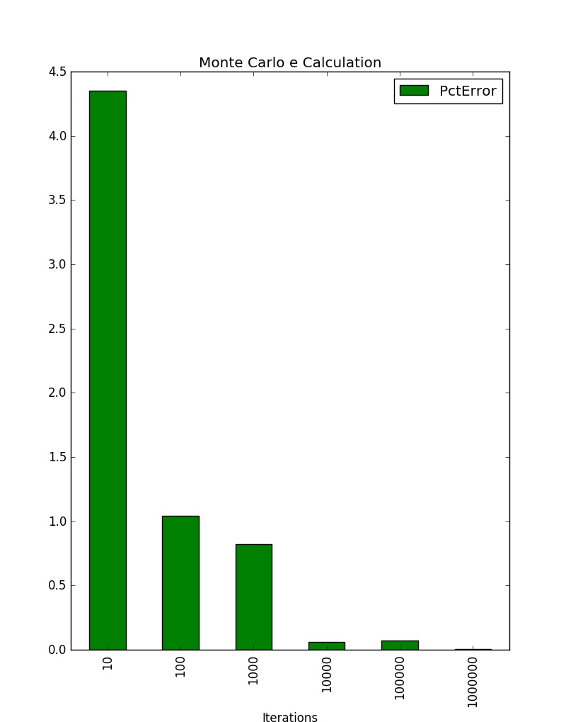
    frame.plot(x='Iterations', y='PctError', kind='bar', title='Monte Carlo e Calculation', color=['g'])
    plt.show()

Results

   Iterations  PctError
0          10  4.351345
1         100  1.040430
2        1000  0.819703
3       10000  0.058192
4      100000  0.072773
5     1000000  0.005512

Fire Ant Simulation

This last simulation is admittedly contrived and likely less than scientifically accurate.  The focus is on the Monte Carlo method.  However, I can say I have some first-hand experience with this model via ~20 years spent in Texas for under-grad work and various military assignments.  For those unfamiliar with fire ants - they are a uniquely offensive member of the animal kingdom.  They bite + sting and are extremely aggressive when disturbed.  Fire ants are in never-ending abundance in Texas.  On that note - I used some fire ant data from this Texas A&M website

This simulation is a model of a typical residential backyard and the fire ant population therein.  The question to be answered:  How long can I sit in my backyard until at least one fire ant is tearing me up?

Diagram of the model below:
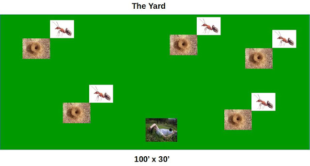
Rude awakening imminent

Model Assumptions

  • 100' x 30' = 3000 sq ft 'yard'
  • 5 ant mounds in the yard
  • 500K ants
  • Ant mounds are randomly distributed in yard
  • Ants are randomly distributed amongst the mounds.
  • All ants start the simulation at their home mound position.
  • Ants have 2 states in the model.  Foraging or attacking.
  • 1 human exists in the model.  The human is randomly positioned in the yard with the assumption they will not sit directly on a mound.  This assumption is a partial deviation from reality to ensure statistically interesting experiments.  I've personally sat on a fire ant mound (inadvertently).  I don't recall it being statistically interesting.
  • Ants move 3 inches/second, or 1 foot in 4 seconds.
  • Time steps in the model are 4 seconds
  • Ants on the move ('foraging') will randomly choose among 8 possible directions at each time step.  This provides the randomness of the model.
  • Ants on the move will stay the course in 1 direction for an entire time step (same direction for 1 foot/4 seconds)
  • Ants can't leave the boundaries of the yard.  An attempt to do so results in no movement for that time step.
  • Only 50% of the ant population makes a move in any given time step.  The rest are idle for that time step.
  • Once an ant gets within 1 foot of the human position, it starts attacking.  An attacking ant never leaves the 'attacking' state.  Again, I can attest from personal experience that this represents reality.
  • The simulation ends when at least 1 ant achieves the 'attacking' state.

Python Implementation

class Yard(object):
    length = 100 #3000 sq ft yard
    width = 30
    numMounds = 5
    numAnts = numMounds * 100000 #100K ants per mound
    pctAntsActive = .5 #percentage of the ants moving at any given time step
    
    def __init__(self):
        random.seed()
        self.__setMounds()
        self.__setAnts()
        self.__setHuman()
        
    def __setMounds(self): 
        self.moundPositions = []
        xlist = random.sample(range(0, Yard.length+1), Yard.numMounds)
        ylist = random.sample(range(0, Yard.width+1), Yard.numMounds)
        for i in range(Yard.numMounds):
            mound = (xlist[i], ylist[i])
            self.moundPositions.append(mound)
    
    def __setAnts(self):
        self.ants = []
        for _ in range(Yard.numAnts):
            mound = random.choice(self.moundPositions)
            self.ants.append(Ant(mound))
                
    def __setHuman(self):
        done = False
        while not done:
            x = random.randint(0, Yard.length)
            y = random.randint(0, Yard.width)
            if (x, y) not in self.moundPositions: 
                done = True
            else:
                pass
            
        self.humanPosition = (x, y)
    
    def clockTick(self):
        antsAttacking = 0
        activeAnts = random.sample(range(0, Yard.numAnts), int(Yard.numAnts*Yard.pctAntsActive))
        
        for ant in activeAnts:
            state = self.ants[ant].move(self.humanPosition)
            if state == 'attacking':
                antsAttacking += 1
                break
            else:
                pass
        
        return antsAttacking
Line 1:  Class definition of the "Yard"
Lines 2-6:  Class variables capturing some the model assumptions
Lines 8-12:  Class initializer which sets up the model.
Lines 14-20:  Function to randomly distribute the ant mounds in the yard.
Lines 22-26:  Function to create the ant objects and randomly distribute them among the mounds.
Lines 28-38:  Function to randomly position the human in the yard, but not on top of a mound.
Lines 40-52:  Main driver of the simulation.  Provides a four-second time step during which a random 50% distribution of ants make a one-foot move.  Function returns the number of ants that reached the 'attacking' state in that time step.

class Ant(object):
    __directions = ['NW', 'N', 'NE', 'E', 'SE', 'S', 'SW', 'W']
    
    def __init__(self, position):
        self.position = position
        self.state = 'foraging'
    
    def __checkAttack(self, humanPosition):
        distance = math.sqrt((self.position[0] - humanPosition[0])**2 + (self.position[1] - humanPosition[1])**2)
        if distance <= 1:
            return 'attacking'
        else:
            return 'foraging'
    
    def move(self, humanPosition):
        if self.state == 'foraging':
            direction = random.choice(Ant.__directions)
              
            if direction == 'NW':
                x = self.position[0] - 1
                y = self.position[1] + 1
            elif direction == 'N':
                x = self.position[0] 
                y = self.position[1] + 1
            elif direction == 'NE':
                x = self.position[0] + 1
                y = self.position[1] + 1
            elif direction == 'E':
                x = self.position[0] + 1
                y = self.position[1] 
            elif direction == 'SE':
                x = self.position[0] + 1
                y = self.position[1] - 1
            elif direction == 'S':
                x = self.position[0] 
                y = self.position[1] - 1
            elif direction == 'SW':
                x = self.position[0] - 1
                y = self.position[1] - 1
            elif direction == 'W':
                x = self.position[0] - 1
                y = self.position[1]
            else:
                pass
              
            if x >= 0 and x <= Yard.length and y >= 0 and y <= Yard.width:
                self.position = (x, y)
            else:
                pass
            self.state = self.__checkAttack(humanPosition)
        else:
            pass
        
        return self.state
Line 1:  Ant class definition
Line 2:  Class variable containing a list of the 8 different directions an ant can move
Lines 4-6:  Class initializer setting an ant's initial position and state.
Lines 8-13:  Private class function for determining if an ant is within 1 foot of the human's position.  If so, the ant's state is set to 'attacking.'
Lines 15-54:  Resets an ant position by 1 foot in a randomly chosen direction.  If the resulting position is outside of the yard boundaries, the ant remains stationary.  Returns the new state of the ant based on its new position.
def simulation(): 
    yard = Yard()
    seconds = 0
    numAttacking = 0
    
    while numAttacking == 0:
        numAttacking = yard.clockTick()
        seconds += 4
    
    return seconds
Lines 1-10:  Global function providing simulation driver.  Sets up the 'yard' and runs a clock until at least 1 ant is attacking the human.

if __name__ == '__main__': 
    simIters = [25,50,75,100]
    avg = {}
    
    for iters in simIters:
        tot = 0
        pool = mp.Pool()
        results = []
        for _ in range(iters):
            results.append(pool.apply_async(simulation))       
        pool.close()
        pool.join()
        for res in results:
            tot += res.get()
        avg[iters] = round(tot / iters)
        print(iters, avg[iters])
    
    
    frame = pd.DataFrame(data=list(avg.items()), columns=['Iterations', 'Seconds'])
    frame.sort_values(by='Iterations', inplace=True)
    frame.reset_index(inplace=True, drop=True)
    print(frame)
    frame.plot(x='Iterations', y='Seconds', kind='bar', title='Monte Carlo Fire Ant Attack Simulation', color=['r'])
    plt.show()        
Lines 2-16:  Sets up a loop that proceeds through 4 different iteration runs of the simulation (25,50,75,100) and creates a multiprocessing pool to run them.  Run time of each simulation is stored for its particular iteration count and then averaged.
Lines 19-24:  Sets up a pandas data frame with the results and display a bar graph.

Results

25 198
50 189
75 121
100 166
   Iterations  Seconds
0          25      198
1          50      189
2          75      121
3         100      166

These simulations maxed out all four cores on my machine for lengthy periods of time.  My guess would be if I were to run higher iteration counts, the attack time would settle somewhere around 150 seconds as that appears to be the trend with these 4 trials.


Source: https://github.com/joeywhelan/montecarlo

Copyright ©1993-2024 Joey E Whelan, All rights reserved.

Sunday, November 19, 2017

Crypto Digest Collisions


Summary

Proof-of-work is a critical component of the various crypto coin variants in use today.  In a nutshell, the blockchain algorithms that form the basis of crypto coins require participants to complete a provable amount of computation before a transaction can be added to the chain.  Partial hash collision is one such proof of work.

The post covers a toy implementation of partial hash collision.

Background

The basis for this proof-of-work method is hash digests.  An input string is processed through a cryptographically-strong function that outputs a fixed-length and unique hash value for that given input string.  Given a strong hash algorithm, it should be computationally unfeasible to find two input strings that create the same hash digest - also known as collision resistance.

Collisions on the full bit-length of a hash may be unfeasible, but collisions on a subset of the bits can be accomplished.  There are no known short-cuts to finding a collision but trial and error - submitting a different input string to a hash algorithm, over and over.  The typical partial hash collision method takes a string as input, concatenates a number to that string, then tests the high-order bits of the resulting hash.  If the necessary number of high-order bits are all 0, a solution has been found.

Example:  Say a given hash algorithm outputs a 10-bit hash and we want to find string with given input that results in the first 4 bits all equal to 0.  There are 2**10 total unique hashes available in this algorithm.  There are 2**6 hashes where the first 4 bits are 0.  In general, we would have to try 2**4 (16) inputs to the hash algorithm to find a solution.  Real world implementations deal with 160/256 bit hashes and collision lengths of >20 bits.

Implementation

Single Process

totalBits = 256  
collisionBits = 23 
mask = (1<<totalBits) - (1<<totalBits-collisionBits)
textInput = None

def singleProcessHash(text):
    count = 0    
    ti = time.time()
    
    while True:
        msg = text + ':' + str(count)
        dig = hashlib.sha256(msg.encode(encoding='utf_8', errors='strict')).hexdigest()
        res = int(dig,16) & mask
        if res == 0:
            break   
        count+=1
            
    print('Single-process run time: {:0.4f}'.format(time.time()-ti))
    print ('Message: ', msg)
    return msg
Lines 1-2:  Total bit length of the hash and the number of required high-order bits to be set to 0.  SHA-256 outputs a 256-bit hash.  For this example, the 23 high-order bits have to be 0 for a valid solution string.
Line 3:  Constucts a 256-bit mask with the 23 high-order bits set to 1.  All other bits are 0.
Lines 10-16: Brute-force loop that successively concats a number to the input text, hashes it thru SHA-256, and then does a bit-wise AND against the mask to test if the 23 high-order bits are all 0.  If the result isn't a partial collision, increment the counter and continue to loop.

Multiple Processes

def init(text):
    global textInput
    textInput = text
    
def findCollision(arg):
    global textInput
    msg = textInput + ':' + str(arg)
    hsh = hashlib.sha256(msg.encode(encoding='utf_8', errors='strict')).hexdigest()
    res = int(hsh,16) & mask
    if res == 0:
        return msg

def multiProcessHash(text):
    mult = 1
    numValues = 10**6
    chunkSize = math.ceil(numValues/mp.cpu_count())
    found = False
    msg = None
    ti = time.time()
   
    pool = mp.Pool(initializer=init, initargs=[text])
    while not found: 
        sample = range(numValues*(mult-1), numValues*mult)
        mult += 1
        results = pool.imap_unordered(findCollision, sample, chunkSize)
        for msg in results:
            if msg:
                pool.terminate()
                pool.join()
                found = True
                break

    print('Multi-process run time: {:0.4f}'.format(time.time()-ti))
    print('Message: ', msg)
    return msg
Lines 1-3:  Init function setting the text argument for each of the worker processes in the pool. Unfortunate aspect of Python, but use of globals is the most straight-forward way to accomplish this.
Lines 5-11:  Collision test function performed by each of the worker processes.
Line 15:  Variable to set up 1M values to be sent to the pool per iteration.
Line 16:  Chunk up those 1M test values evenly amongst the worker processes.  One worker per CPU.
Lines 21-31:  Set up the worker pool and loop through successive 1M value batches of samples until a partial collision is found.

Results

This was tested on a quad-core machine with hyper-threading (8 logical CPU's).
if __name__ == '__main__':
    singleProcessHash(string.ascii_uppercase)
    print()
    multiProcessHash(string.ascii_uppercase)  
Single-process run time: 18.9084
Message:  ABCDEFGHIJKLMNOPQRSTUVWXYZ:7201566

Multi-process run time: 6.7886
Message:  ABCDEFGHIJKLMNOPQRSTUVWXYZ:7201566


Copyright ©1993-2024 Joey E Whelan, All rights reserved.

Friday, September 8, 2017

AI-Driven Investing with Lending Club - Part 5: Ensembling


Summary

This is the fifth installment in the series I've written on my experience implementing a machine learning engine for selecting loans for investment from Lending Club.  In this article, I'll discuss and apply a couple techniques for combining the results of multiple classifiers.
There's quite a bit of literature out there on ensembling as it has been a popular (and winning) technique in Kaggle competitions.  In a nutshell, ensembling attempts to combine the strengths of multiple classifiers to produce a classifier that is better than its parts.

The simplest ensemble, and in fact has an out-of-box implementation in scikit-learn - VotingClassifier, is voting.  In 'hard' voting, the majority prediction from multiple classifiers is taken to be the final prediction.  In 'soft' voting, the probabilities from multiple classifiers are summed to come up with the final prediction.

A more complex ensembling technique is known as stacking (sometimes also referred to as 'blending').  In this model, classifiers are 'stacked' in levels.  The outputs of the classifiers in the lower levels become the inputs to the classifier(s) in the upper levels.

An interesting variation of stacking was developed for the Netflix Prize competition in 2009 and was in fact the 2nd place winner.  Feature-weighted Linear Stacking takes 'meta-features' and combines them via linear regression to a stacked model.  Video here from Joe Sill, a member of the 2nd place team, describing the technique.

Implementation

I decided to approach this with a Python class (Ensemble) that implements both voting and stacking.  I settled on four classifiers:  GBC, MLP, RBM, and SVD.  I ran all four through a grid-search to find a good parameter set for each classifier for my particular data set.

Below is some code that tests each classifier in isolation and prints out a Pearson correlation matrix for the four classifiers.  Good classification performance per classifier and low-correlation between classifiers are goals for an ensemble.
        pool = mp.Pool(processes=mp.cpu_count())
        results = []

        for name, clf in self.estimators.items():
            try:
                self.estimators[name] = joblib.load('./models/' + name + '.pkl')
            except FileNotFoundError:  
                logging.debug('{} not pickled'.format(name))    
                results.append(pool.apply_async(lvl1_fit, args=(clf, name, features_train, labels_train)))           
           
        pool.close()
        pool.join() 
        for result in results:
            item = result.get()
            name = item['name']
            self.estimators[name] = item['fittedclf']
        
        #Print confusion matrix and score for each clf.  
        corr_list = []
        clf_list = []
        for name, clf in self.estimators.items():
            preds = clf.predict(features_test)
            self.confusion_matrix(name, labels_test, preds)
            print()
            self.classification_report(name, labels_test, preds)
            corr_list.append((name, preds))
            clf_list.append(name)
        
        #Print a matrix of correlations between clfs
        frame = pd.DataFrame(index=clf_list, columns=clf_list)
    
        for pair in itertools.combinations(corr_list,2):
            res = pearsonr(pair[0][1],pair[1][1])[0]
            frame[pair[0][0]][pair[1][0]] = res
            frame[pair[1][0]][pair[0][0]] = res
        frame['mean'] = frame.mean(skipna=True,axis=1)
        pd.options.display.width = 180
        print('Correlation Matrix')
        print(frame) 

Lines 1-16: Load up the fitted classifiers.  'estimators' is an OrderedDict of scikit-learn classifier objects.  If the fitted classifiers have already been cached to disk, use that.  Otherwise, fit them from scratch on the training set in a multiprocessing pool.
Lines 18-27:  Generate predictions for each classifier for the test set, then print a confusion matrix and classification report for each.
Lines 29-39:  Generate the Pearson correlation between each pair of classifiers and then organize the results in a matrix.

Excerpt of the output below:
svd Confusion Matrix (66392 samples): 
[[ 8599  4654]
 [22715 30424]]

svd Classification Report
             precision    recall  f1-score   support

    Default       0.27      0.65      0.39     13253
       Paid       0.87      0.57      0.69     53139

avg / total       0.75      0.59      0.63     66392

Correlation Matrix
          gbc       mlp       rbm       svd      mean
gbc       NaN  0.746548  0.603429  0.532055  0.627344
mlp  0.746548       NaN  0.516596  0.538988  0.600711
rbm  0.603429  0.516596       NaN  0.408401  0.509475
svd  0.532055  0.538988  0.408401       NaN  0.493148

Voting

The voting portion is quite simple as it is simply a wrapper around the out-of-box implementation from scikit-learn.

Fitting of the voting classifier below:
        try:
            self.voteclf = joblib.load('./models/voteclf.pkl')
        except FileNotFoundError: 
            ti = time() 
            self.voteclf = VotingClassifier(estimators=list(self.estimators.items()), voting='soft',n_jobs=-1)      
            self.voteclf.fit(features_train, labels_train)
            joblib.dump(self.voteclf, './models/voteclf.pkl') #cache the fitted model to disk
        logging.debug('Exiting __fit_vote()')
Lines 1-9:  If the voting classifier has already been fitted and cached to disk, load it.  Otherwise, fit it from scratch and dump the fitted model to disk.

Prediction with the voting classifier below:
preds = self.__predict_with_threshold(self.voteclf, features)

def __predict_with_threshold(self, clf, features):
        ti = time()
        predictions = Ensemble.__custom_predict(clf.predict_proba(features)[:, MINORITY_POS], \
                                                clf.predict(features), self.threshold)
        return predictions

__custom_predict = np.vectorize(vfunc, otypes=[np.int])

def vfunc(probability, prediction, threshold):
    if probability >= threshold:
        return MINORITY_CLASS
    else:
        return prediction
Line 1:  Pass the fitted voting classifier to a custom predict function that operates with thresholds.
Lines 3-15:  Custom prediction function that uses a threshold to decide whether the minority class should be chosen as the prediction.  This is a method to deal with unbalanced classes.

Stacking

The stacking implementation is significantly more complex.  Fitting, for example, requires fitting of each of the four 1st level classifiers and then fitting each of them in K-Fold cross-validation to generate the training data for the 2nd level classifier.  I'm using an unbalanced data set from Lending Club that has over 600K records.  Balancing that takes its size to a ~1M records.  Fitting on data sets of this size mandates use of multiprocessing and caching of the fitted classifiers to disk.

        pool = mp.Pool(processes=mp.cpu_count())
        results = [] #array for holding the result objects from the pool processes
        
        #fit 1st level estimators with a multiprocessing pool of workers
        for name, clf in self.estimators.items():
            try:
                self.estimators[name] = joblib.load('./models/' + name + '.pkl')
            except FileNotFoundError:  
                logging.debug('Level 1: {} not pickled'.format(name))    
                results.append(pool.apply_async(lvl1_fit, args=(clf, name, features_train, labels_train)))           
           
        pool.close()
        pool.join() 
       
        for result in results:
            item = result.get()
            name = item['name']
            self.estimators[name] = item['fittedclf'] #reassign a fitted clf to the estimator dictionary
        
        #fit 2nd level estimator with a multiprocessing pool of workers that perform a k-fold cross-val of 
        #training data
        pool = mp.Pool(processes=mp.cpu_count())
        del results[:]
        try:
            self.lrc = joblib.load('./models/lrc.pkl') #try to load the 2nd level estimator from disk
        except FileNotFoundError: #2nd level estimator not fitted yet
            logging.debug('Level 2: LRC not pickled') 
            folds = list(StratifiedKFold(n_splits=5).split(features_train, labels_train)) 
            #define a frame for holding the k-fold test results of the 1st level classifiers
            lvl2_frame = pd.DataFrame(index=range(0,len(features_train)), 
                                      columns=list(self.estimators.keys()))  
            lvl2_frame[LABEL_COL] = labels_train  
             
            #launch multiprocessing pool workers (1 per fold) that fit 1st level classifers and perform
            #predictions that become the training data for the 2nd level classifier (Logistic Regression)   
            for name,clf in self.estimators.items():
                fold = 1
                for train_idx, test_idx in folds:
                    X_train, X_test = features_train[train_idx], features_train[test_idx]
                    Y_train = labels_train[train_idx]
                    col_loc = lvl2_frame.columns.get_loc(name)
                    results.append(pool.apply_async(lvl2_fit, args=(clf, name, fold, test_idx, \
                                                                    col_loc, X_train, Y_train, X_test)))
                    fold = fold + 1
            pool.close()
            pool.join() 
           
            #fetch worker results and put them into a frame that will be used to train a 2nd Level/Logistic
            #regression classifier
            for result in results:
                item = result.get()
                name = item['name']
                test_idx = item['test_idx']
                col_loc = item['col_loc']
                preds = item['preds']
                lvl2_frame.iloc[test_idx, col_loc] = preds

            self.lrc = LogisticRegression(C=2.0)
            ti = time()
            X = lvl2_frame.drop(LABEL_COL, axis=1).values
            Y = lvl2_frame[LABEL_COL].values
            self.lrc.fit(X, Y)     
            logging.debug('LRC fit time: {:0.4f}'.format(time()-ti))
            joblib.dump(self.lrc, './models/lrc.pkl')  #cache the Logistical Regressor to disk

def lvl1_fit(clf, name, features_train, labels_train):
    logging.debug('Entering lvl1_fit() {}'.format(name))
    ti = time()
    fittedclf = clf.fit(features_train, labels_train)
    logging.debug('{} fit time: {:0.4f}'.format(name, time()-ti))
    joblib.dump(fittedclf, './models/' + name + '.pkl') #cache the fitted model to disk
    logging.debug('Exiting lvl1_fit() {}'.format(name))
    return {'name': name, 'fittedclf': fittedclf}

def lvl2_fit(clf, name, fold, test_idx, col_loc, features_train, labels_train, features_test):  
    logging.debug('Entering lvl2_fit() {} fold {}'.format(name, fold))
    ti = time()
    clf.fit(features_train, labels_train)
    logging.debug('{} fold {} fit time: {:0.4f}'.format(name, fold, time()-ti))
    preds = clf.predict_proba(features_test)[:, MINORITY_POS]
    logging.debug('Exiting lvl2_fit() {} fold {}'.format(name, fold))
    return {'name': name, 'test_idx' : test_idx, 'col_loc' : col_loc, 'preds' : preds}
Lines 1-18:  Attempt to load fitted classifiers from disk.  If they don't exist, use a pool of workers to fit each classifier to the full training set.
Lines 20-56:  With K-Fold (5 folds) cross validation, fit each of the classifiers and then generate predictions with the test set in that fold.  Save the predictions to a data frame.
Lines 58-64:  Fit the 2nd level classifier (Logistic Regression) to the predictions from the 1st level classifiers.  Dump the fitted Logistic classifier to disk.
Lines 66-73:  Function for fitting the 1st level classifiers and dumping them to disk.
Lines 75-82:  Function called within the K-folding for fitting 1st level classifiers and generating predictions to use to train the 2nd level classifier.

Generating predictions from the stacked ensemble requires running the features through all of the 1st level classifiers and then sending their output (predictions) to the 2nd level classifier - Logistic Regression.
 def __predict_stack(self, features):
        lvl1_frame = pd.DataFrame()
        #1st level predictions
        for name, clf in self.estimators.items():
            lvl1_frame[name] = clf.predict_proba(features)[:, MINORITY_POS]
            
        #2nd level predictions
        preds = self.__predict_with_threshold(self.lrc, lvl1_frame.values)
   
        return preds

Source:  https://github.com/joeywhelan/Ensemble/

Copyright ©1993-2024 Joey E Whelan, All rights reserved.